Why Behind-the-Meter Power Emissions Belong in Scope 2

Key Takeaways

• The opportunity: Clean, firm power is a strategic priority for large electricity buyers. Natural gas-fired generation equipped with carbon capture and storage (CCS) is emerging as a key tool in meeting this demand. The existing gas-fired power fleet in the US should be assessed to identify plants well-positioned for carbon capture retrofits that would benefit grid decarbonization. 
• The challenge: The climate benefits of CCS-equipped natural gas plants depend entirely on how often they actually run. Adding carbon capture technology increases the cost to operate the equipment. These higher running costs can make the plant less competitive in auctions where the grid operator picks the cheapest power first. Without mechanisms to keep these plants running continuously, they may be outbid by cheaper, higher-polluting plants, causing grid-wide emissions to stay the same or even increase. 
• The solution: Hyperscalers and other large energy buyers are creating a robust market for clean, firm power. By paying a "clean, firm premium" through long-term offtake agreements, these buyers can offset the higher operational costs of CCS, ensuring these plants are continuously utilized. This corporate leadership not only maximizes the grid-wide climate impact of each retrofit but also provides an important hedge against policy volatility, securing the investment case for clean innovation even when the future of subsidies like the 45Q tax credit is uncertain.

We Need Clean, Firm Power Now

The market signals for clean, firm power are clear. Meta’s nuclear energy projects and Microsoft’s Crane Clean Energy Center demonstrate growing interest in reliable, low-carbon electricity to support the rapid expansion of AI. Similar commitments by Google and Meta to advanced geothermal power also illustrate this trend. 

One of the near-term options to meet this demand is natural gas with carbon capture and storage (CCS). As explored by Relae (formerly Carbon Direct), retrofitting existing gas facilities offers a path to reliable baseload power with low direct emissions, leveraging existing infrastructure to bypass the years-long delays typical of new grid interconnections. 

Recent initiatives from Google and Calpine are already working to prove this concept at scale. This type of corporate leadership is driving the market; over the last decade, voluntary corporate procurement led to more than 40% of new clean energy capacity in the US. Further, recent procurement decisions illustrate that these players are willing to pay a “clean, firm premium” to secure round-the-clock, low-emissions sources of power.

Why Systems-Level Analysis Matters for CCS

While news of corporate procurements often makes headlines, recent analysis finds the number of supply contracts for natural gas power with CCS may outpace the number of secured offtake agreements. Without a power purchase agreement (PPA) to ensure competitive operation, or strong policy support, a generator may need to operate as a “merchant plant” in power markets, competing solely on cost.

A power plant’s ultimate climate impact is determined primarily by how it is positioned in the market, not just its facility-level technology. 

How Power Markets Determine Which Plants Run

Understanding the potential of CCS to deliver clean, firm power and grid-wide decarbonization requires looking beyond the technology performance at a single facility. A retrofitted plant does not operate in isolation; its impact depends on how it interacts with the broader power market’s merit order.

The merit order is the ranking system in competitive power markets where the grid operator dispatches the cheapest offers first. Since carbon capture units are energy-intensive, the retrofitted natural gas plant incurs higher operating costs. This cost increase can inadvertently price the lower-emitting plant out of the market. Without mechanisms to ensure continuous utilization, the CCS plant is potentially outbid by cheaper, more carbon-intensive resources. This creates a risk of increased overall grid emissions.

To illustrate this dynamic, we’re sharing the results of our detailed grid modeling analyses of the Electric Reliability Council of Texas (ERCOT), which serves most of Texas, and the Southwest Power Pool (SPP), which covers parts of 14 states across the central US. Our analysis highlights the value of corporate “clean, firm premiums” in achieving maximum climate benefit and mitigating policy risk present in government subsidy support. 

This type of systems-level grid modeling is necessary in understanding how facility-level reductions translate into real climate benefits. Support to incentivize continuous operation, such as corporate offtake agreements or the 45Q tax credit, is key to ensuring that retrofitting a gas power plant with CCS reduces overall grid emissions. 

Offtake Agreements and Policy Support as Solutions

Power offtake from CCS retrofitted gas plants can meaningfully reduce system-level emissions. By directly matching electricity demand with the supply of power, large energy buyers – the offtakers – ensure the power plant is effectively utilized. This type of arrangement helps ensure any changes to reduce emissions intensity at the facility level translate into broader emissions reductions on the grid.

For these offtakers, the decision to pay a premium for clean power is driven by the goal of additionality – ensuring their procurement has a measurable, additional emissions reduction impact. Beyond physical energy, buyers secure Energy Attribute Certificates (EACs) for CCS, which serve as the verified proof of low-carbon generation required to satisfy corporate zero-emissions targets. As seen in the recent Google and Calpine agreement, these certificates allow buyers to claim the specific climate benefit of the CCS retrofit, justifying a premium over standard wholesale market rates to secure firm, clean delivery.

In the absence of offtake agreements, policy frameworks like the 45Q tax credit (up to $85 per ton of CO₂ sequestered) serve a similar function by offsetting production costs.

However, access to this credit is not a guarantee and carries operational hurdles. To unlock the full credit value, facilities must meet stringent prevailing wage and apprenticeship requirements. Furthermore, the credit is limited to a 12-year window once the facility is placed in service, and requires construction to commence by 2033.

Beyond these eligibility requirements, the long-term outlook for 45Q involves inherent uncertainty. Recent regulatory shifts, including potential changes to the Greenhouse Gas Reporting Program (GHGRP), pose risks to the verification mechanisms required to substantiate captured tons. 

Corporate offtake agreements offer a crucial private-sector complement to this landscape; they provide a stable revenue model independent of policy cycles, ensuring the investment case remains robust over the full life of the asset.

Understanding the Merit Order in Power Markets

Most US power plants operate in competitive deregulated markets, where grid operators dispatch generators based on their marginal cost of production – the cost of generating one additional unit of electricity. The operator ranks these offers from lowest to highest price, creating the "merit order.”

In these auctions, the cheapest resources (typically renewables and base load) are dispatched first. Progressively more expensive units (gas and peaking plants) are called upon until demand is met. The price of the final, most expensive unit required sets the market-clearing price received by all generators in that period. 

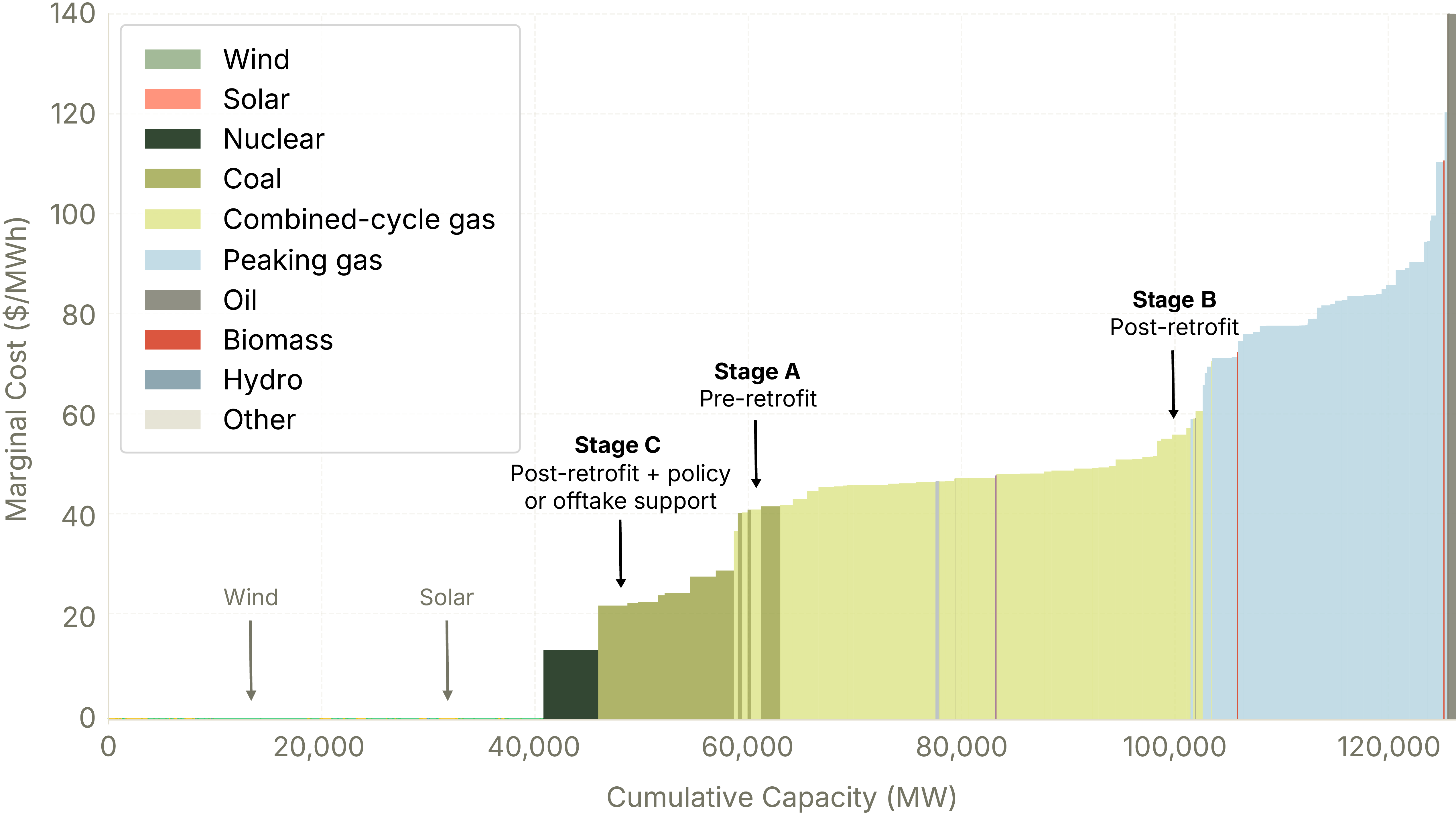
The Figure below shows an example generation merit order in the ERCOT energy market.

Case Study: How Support Structures Influence Dispatch

The merit order figure illustrates a hypothetical scenario for a natural gas generator, showing how its market position changes based on technical and policy variables:

• Pre-Retrofit (Stage A): The plant operates with standard marginal costs, sitting competitively in the middle of the supply stack.
• Post-Retrofit (Stage B): Retrofitting with CCS introduces higher operating costs due to the energy-intensive nature of carbon capture. Without external support, the plant’s marginal cost increases (A to B), making it less competitive. The retrofitted plant may be utilized less while cheaper units are dispatched to meet demand.
• Post-Retrofit + policy or offtake support (Stage C): Financial support, whether through the 45Q tax credit (approx. $33/MWh¹) or a corporate offtake agreement, can effectively offset the plant’s higher operational costs (B to C). This effect restores the plant’s competitiveness, ensuring it dispatches consistently.

Testing This With Grid Modeling

At Relae, we apply state-of-the-art grid analysis tools to answer these and more complex analytical questions related to the future energy system. Our custom modeling framework has been used to simulate clean power strategies, assess data center demand response programs, and understand how procurement decisions today impact the future energy system.

While the theoretical impact of a CCS retrofit, a PPA agreement, and the 45Q tax credit on a plant’s dispatch is clear, it’s important to put the theory to the test by modeling their effects on system-wide emissions.

Our Modeling Approach

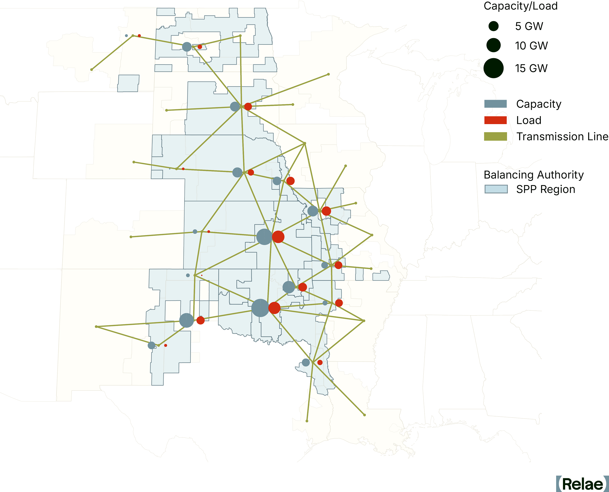
Because each grid region has distinct power plants and load requirements, they must be modeled separately. For this analysis, we chose to model the ERCOT and SPP power markets to determine the region-specific, grid-wide emissions impact of hypothetical CCS retrofits of natural gas power plants. 

As part of this modeling, we:

• Deployed detailed hourly simulation: We used our custom PyPSA-USA grid model to produce a set of hourly simulations of the ERCOT and SPP electricity markets.²
• Identified suitable retrofits: We identified suitable combined cycle gas power plants for a CCS retrofit in each of the markets, based on key commercial and operational criteria, including size, age, generation profile, and proximity to CO₂ transport/storage.
• Modeled plant and energy assumptions: To reflect the retrofit, we adjusted generator cost and energy use for the identified plants (up to 1.4 GW capacity), fitting all combustion turbines with capture and requiring each plant to consume 20% more fuel per unit of electricity produced to power CCS.³
• Carried out comparative scenario analysis: We simulated several scenarios, including (1) pre-retrofit, business-as-usual, (2) post-retrofit, with and without a PPA, and (3) post-retrofit, with and without the 45Q tax credit, to isolate the impact of different procurement agreements and policy landscapes on grid-wide emissions. 

What Our Analysis Reveals

Results of this analysis reveal how CCS deployment in the power grid interacts with market economics and the role mechanisms that drive high utilization of CCS retrofit plants can have in ensuring system-wide emissions reductions:

CCS With a Firm Offtake Agreement Can Significantly Reduce Grid-Wide Emissions

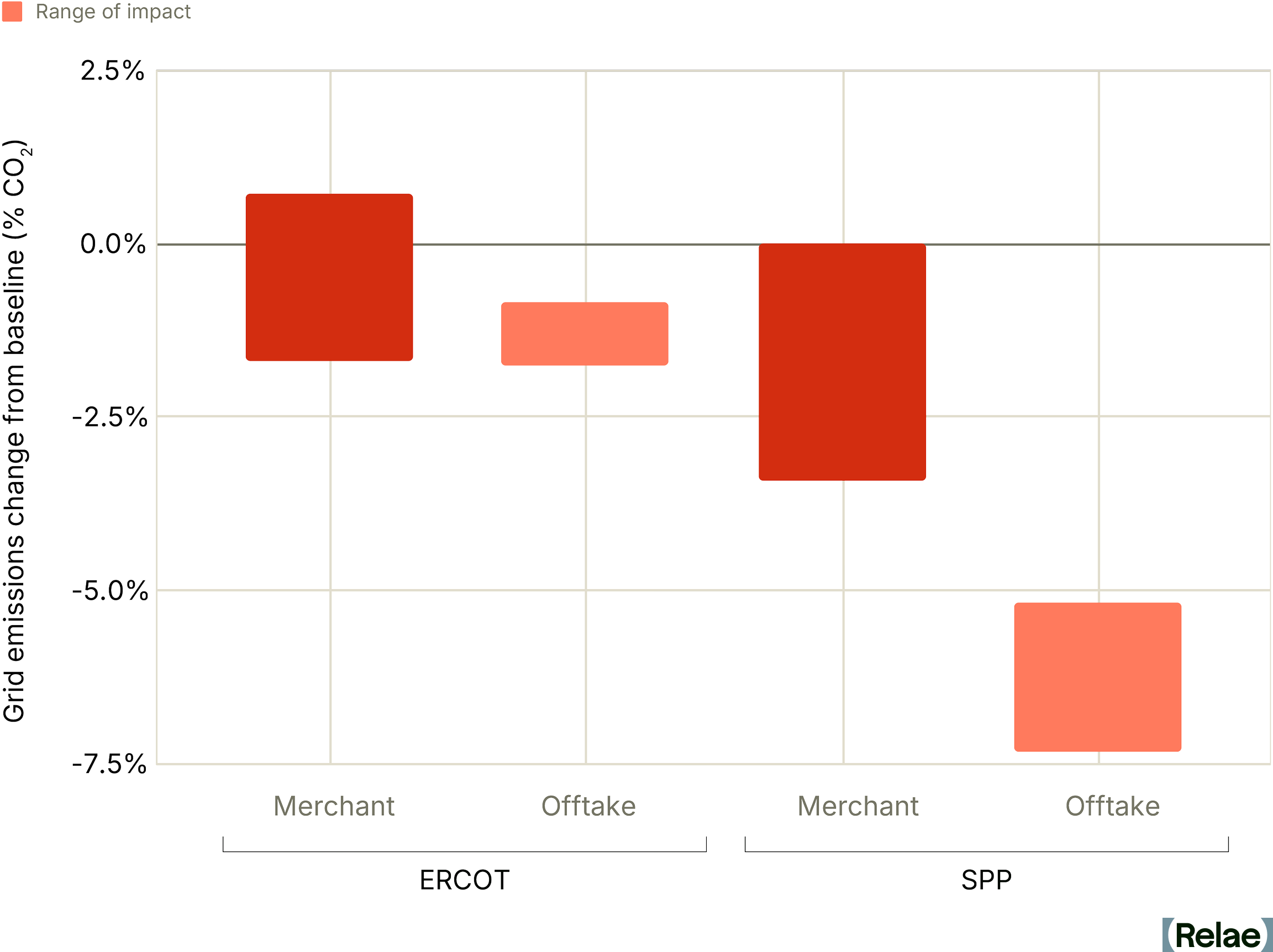
Pairing a retrofitted plant with a dedicated offtaker can drive meaningful emissions reductions in both ERCOT and SPP compared to business-as-usual (-0.8% to -1.7% CO₂ in ERCOT; -5.2% to -7.3% CO₂ in SPP). Under these arrangements, system-wide emissions fall because the PPA acts as an operational anchor, ensuring the retrofitted plant maintains high utilization rates despite its higher running costs. Ensuring the plant stays utilized prevents the grid from reverting to more carbon-intensive generation to fill the gap.

Our analysis finds the value of the operational “clean, firm premium” for natural gas with CCS power is up to $60 per MWh. This value varies by hour, region and scenario but results generally align with our previous estimate of a $30 per MWh value associated with this type of generation. Other estimates put this value between $19 and $72 per MWh.

CCS Without an Offtake Agreement Can Reduce Emissions, But Is More Reliant on Policy Support

Without a dedicated offtake agreement or policy support, retrofitting natural gas plants with CCS runs the risk of a small increase in grid emissions (+0.7% CO₂ in ERCOT; -0.0% CO₂ in SPP). System-wide emissions are higher because other power plants displace the plants with carbon capture. The higher operational costs of CCS mean the CCS plants have a less competitive place in the merit order and run for fewer hours in the year.

The story changes with the application of 45Q, and grid-wide emissions are lower for both ERCOT and SPP (-1.7% CO₂ in ERCOT; -3.4% CO₂ in SPP). Access to the 45Q tax credit improves each CCS plant’s position in the merit order, meaning that it runs for more hours and successfully displaces higher-emitting generation with clean, firm power.

The Path Forward for Clean, Firm Power

Our analysis illustrates that in competitive power markets, the overall carbon emissions impact of natural gas generation with CCS cannot be measured solely at the power plant level. While clean, firm power remains a strategic priority for large electricity buyers, and CCS is a key tool to meet this demand, the overall climate value of a successful retrofit is linked to the availability of offtake agreements and the plant’s position in the merit order. 

A systems-level perspective captures what facility-level analysis misses: how market dynamics determine the true climate impact of decarbonization investments. Support mechanisms for the continuous operation of low-carbon power plants, like PPAs and the 45Q tax credit, are important tools that ensure clean, firm power reaches the grid, effectively bridging the competitiveness gap.

Frequently Asked Questions 

How can companies ensure CCS retrofits actually reduce grid-wide emissions? 

By securing the plant’s dispatch through a long-term offtake agreement, or by utilizing a policy incentive like 45Q. Relae’s modeling found that offtake agreements have a substantial impact on the emissions reduction potential of CCS retrofits. 

Why would the dispatch decisions of one power plant affect others? 

Power plants dispatch according to marginal cost, and grid stability requires that total supply remain constant at any given moment. So, if one large plant suddenly dispatches less (say, because its operating costs have increased), other potentially dirtier plants may ramp up to fill the gap, increasing total system emissions.

Key Takeaways

• Accurate load forecasting is needed to distinguish and prioritize real demand, align capital deployment, and reduce delays in bringing new power capacity online. Traditional load forecasting was built for predictable, gradual demand growth, not for the scale, uncertainty, and dynamic behavior of data centers. 
• The system-level fix to data-center load forecasting requires probabilistic, more frequent, category-specific methods paired with mandatory data standards and policy alignment. Together, these give planners visibility into the range of possible futures and the likelihood of each. 
• Without that fix, today's forecasts conflate real demand with speculative submissions, reducing accuracy. Inaccurate forecasting in either direction is expensive: underbuild adds friction to economic development; overbuild risks raising retail rates. Both can erode public trust in planning.
• Behind-the-meter generation (BTM) and load flexibility can help achieve speed-to-power in the near term. Just 1% data-center flexibility could unlock 100 GW—more than the entire US nuclear fleet.

Load Growth Is Increasing, Uncertain, and Concentrated

For two decades, US electricity demand was flat. Utilities, transmission planners, and corporate buyers built their planning models around that reality. Then AI workloads changed it.

AI load growth is large, uncertain, and concentrated in major power markets. While load forecasting projections vary across studies, the trajectory is clear: electricity demand is scaling faster than the bulk power grid was designed to handle. Accurate load forecasting is needed to distinguish and prioritize real demand, align capital deployment, and reduce delays in bringing new power capacity online.

On April 30, 2026, Relae (formerly Carbon Direct) hosted a Trellis Group panel on load forecasting in the AI era. Panelists included Derya Eryilmaz, PhD, Vice President of Power Commercialization at Relae; John Miller, Director of Transmission Policy at the Corporate Energy Buyers Association (CEBA); Daniel Padilla, Strategy and Business Development Lead at Emerald AI; and Sam Hodas, Head of US Government Affairs at National Grid. Jake Mitchell, Director of Climate Tech Innovation at Trellis Group, moderated.

The conversation explored where load forecasts fail, what they cost, how to fix them, and near-term solutions to overcome grid constraints. Here is what the panel found.

What Is Load Forecasting?

Load forecasting is the practice of predicting how much electricity will be consumed across a region, at what times, and under what conditions. It informs the major capital and procurement decisions on the grid: where to build transmission, how much generation to procure, what capacity to bid into wholesale markets, and how corporate buyers secure clean, firm power.

Long-term forecasts inform multi-year decisions about transmission and generation. Short-term operational forecasts inform real-time grid operations and trading. The two often sit in separate workflows, but short-term operational forecasts should feed into long-term system planning to improve accuracy as demand patterns shift.

The Bulk Power Grid Is Under Strain

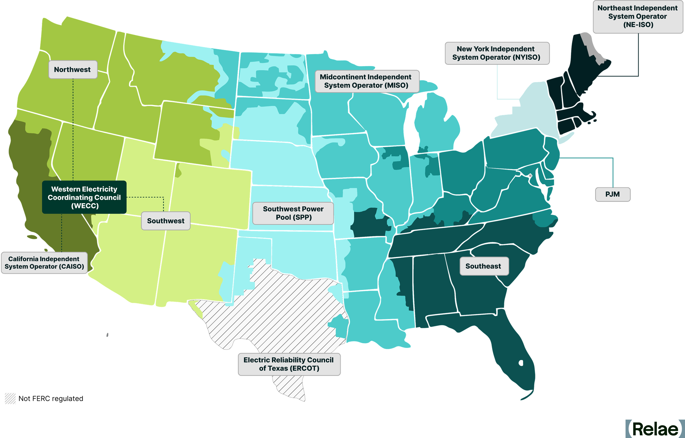
Large power users face constraints on clean, firm power, transmission capacity, multi-year interconnection queues, and aging infrastructure. The strain is most acute in PJM Interconnection (PJM) and the Electric Reliability Council of Texas (ERCOT), the two US markets expected to see the most significant load growth. Each constraint raises the cost of getting load forecasts wrong.

Hodas from National Grid describes the operational reality on the utility side: aging infrastructure inherited from a different demand era. “We’ve got transmission lines that are 70 to 100 years old in New York and Massachusetts, some of the oldest in the country, still in operation.” Replacing or upgrading that infrastructure requires investment, and ratepayers are already pressed. 

Why Today’s Load Forecasts Fail

Traditional load forecasting was built for predictable, gradual demand growth, not for the scale, uncertainty, and dynamic behavior of data centers. 

Most utilities and Independent System Operators (ISOs) produce load forecasts on annual or biannual cycles. They aggregate submissions from individual customers, run that data through a deterministic single-peak load estimate against a single capacity scenario, and pass the consolidated forecast up to regional planners. Regional Transmission Organizations (RTOs) roll those bottom-up utility forecasts into a regional view. 

This worked when demand was flat and predictable. It no longer works with nonlinear growth driven by data centers. Eryilmaz from Relae identifies key structural limitations. 

Four Structural Limitations to Traditional Forecasting Methods

• Over-stating and double-counting. Data centers bid into multiple regions while shopping for power, inflating regional forecasts and blurring the line between real and hypothetical demand—the speculative-load problem.
• Deterministic models (vs probabilistic models). Most planning runs a single peak load estimate against a single capacity scenario, missing the geographic concentration and uncertainty inherent in integrating large loads into the system.
• Aggregated submissions. Utilities report large loads as a single block of gigawatts, with no resolution into workload type, ramp schedule, or operational shape. Planners reverse-engineer peak-demand assumptions rather than measure them.
• Infrequent cadence. Annual or biannual forecasts cannot catch an 80% queue reduction or a multi-gigawatt addition between cycles.

The Speculative-Load Problem

The core challenge in load forecasting is distinguishing real versus hypothetical load. While data center electricity demand is projected to grow by 13-27% annually through 2028, the majority of the projects in the data center queue may not materialize, inflating regional load forecasts.

American Electric Power's Ohio utility (AEP Ohio) introduced a tariff requiring data centers to put up firm financial commitments before getting in line for grid connection. Its interconnection queue dropped from 30 gigawatts to 5.6 gigawatts. More than 80% of the submitted load was speculative: projects that disappeared once commitment became required.

ERCOT shows the same overstatement problem on a larger scale. Roughly 225 gigawatts of data center demand sits in the ERCOT queue against a historic system peak of 85 gigawatts. Texas Senate Bill 6 introduced similar financial obligations for new loads, but those rules apply only to interconnections after 2025, and the cleanup of speculative demand has not yet materialized.

The speculative-load problem shows up in interconnection times. An average new project in PJM can wait 4 to 5 years to become operational. Some of that delay is a real backlog. The rest comes from the inability to distinguish real submissions from speculative ones.

As Eryilmaz puts it, “Load forecasting is actually the center of all of these problems. It is a tool to help planners make the right investment decisions.”

The Cost of Inaccurate Forecasting

As Miller from CEBA notes, “A single misforecasted project can swing a transmission plan by hundreds of megawatts.” Significant inaccuracies can erode public trust in the planning process in two main ways. Underbuilding adds friction to economic development and can limit corporate access to clean power markets. Conversely, overbuilding risks raising retail rates if capacity remains underutilized. 

The goal is to achieve right-sized infrastructure investment. When planning aligns with actual large load growth, it can be net beneficial to retail rates. By spreading fixed costs across more usage, significant new demand can put downward pressure on the rates via the “denominator effect.” 

On the other hand, forecasting variability can distort capacity procurement and interconnection queue prioritization. When load forecasts spike upward, grid operators like PJM have to scramble to buy additional electricity capacity on short notice. These emergency procurements lock in major dollar commitments on the basis of unstable forecast numbers. 

PJM, Midcontinent Independent System Operator (MISO), and Southwest Power Pool (SPP) have also reshaped their interconnection queues to make room for new large loads, but those queue priorities depend on the same forecasts that are unreliable in the first place. 

“There is no substitute for good backbone regional transmission planning,” Miller says. “Full stop. That is the enabler of all of the load growth that we’re talking about.”

BTM Generation and Load Flexibility: A Near-Term Bridge

Hyperscalers’ need for power is way faster than that of utilities and RTOs. Generation alone cannot scale fast enough to meet this new demand, and hyperscalers need speed-to-power.

As Eryilmaz frames it, behind-the-meter generation and load flexibility are interim solutions to the timing mismatch between data center urgency and the grid's slower build cycles. BTM generation and flexibility work differently:

• BTM is power generated on the data center's side of the utility meter, bypassing grid interconnection entirely. The structure gives operators large, reliable blocks of power without waiting years for grid approval.
• Load flexibility is the demand-side approach. A data center modifies its grid draw in response to grid signals. In practice, that can mean curtailing compute workloads during stress events, pre-cooling facilities ahead of a heat wave, drawing from on-site batteries or generators, or shifting workloads to data centers in less-constrained regions.

The Value of Load Flexibility

Relae’s power system modeling quantifies the dollar value of load flexibility in ERCOT. Load flexibility can eliminate forced load shedding risk, even at 40 gigawatts of data center buildout, preventing $5.5 billion in annual consumer welfare losses by curtailing an average of 5% of demand for under 1% of operating hours.

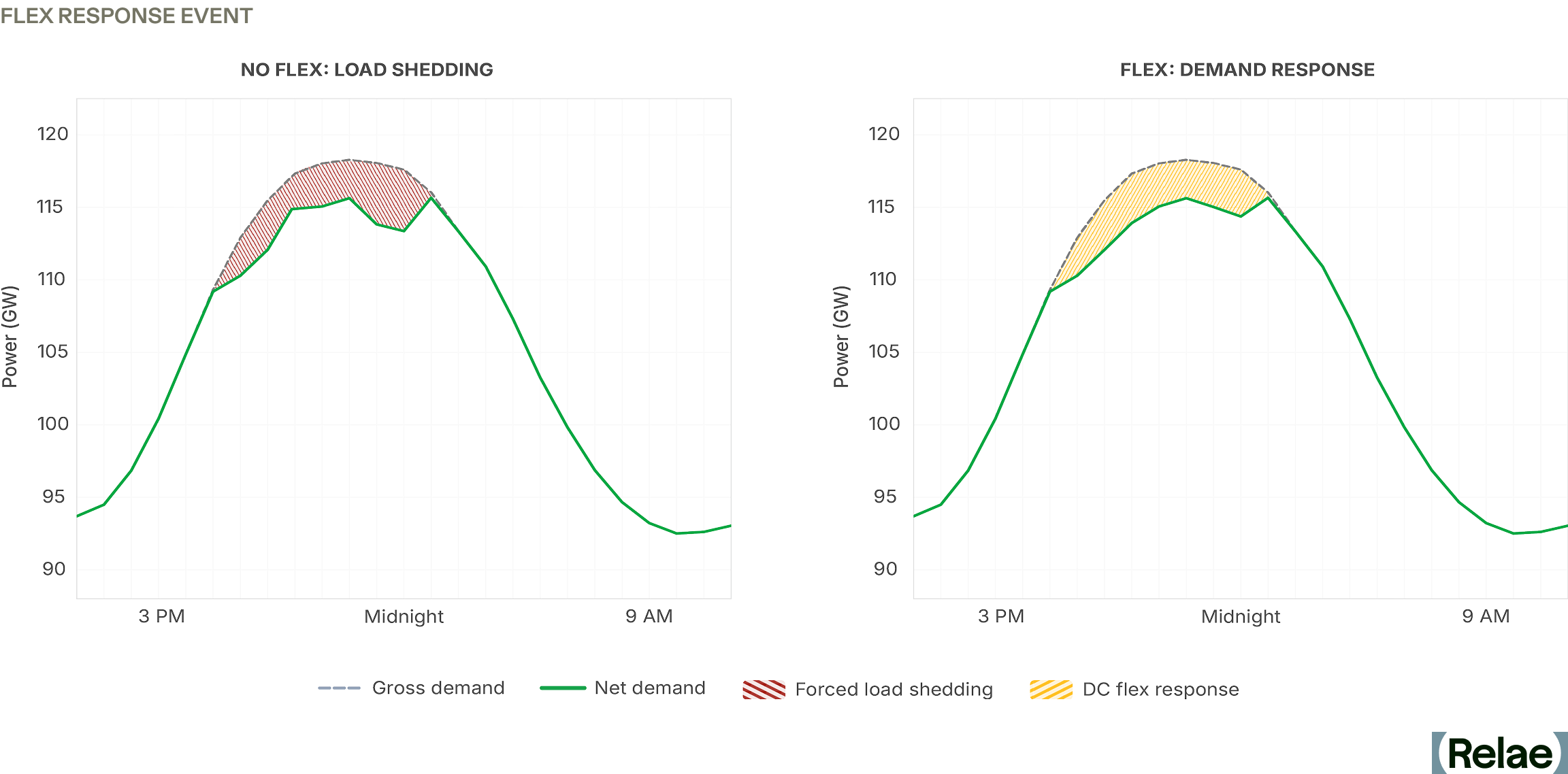
Padilla from Emerald AI reinforces the scale and value of load flexibility: “With just 1% flexibility, we can unlock 100 gigawatts of data centers across the US. That’s more than the entire US nuclear fleet.”

Silicon Valley Power, a municipal utility, is the first US utility to tie flexibility to interconnection speed: flexible data centers get connected faster. NVIDIA, EPRI, Digital Realty, and PJM are partnering on the Aurora AI Factory, the first purpose-built reference design for flexible AI data centers. 

But standardized policy for load flexibility is lagging. Padilla highlights this challenge: “Today, if a data center wants to be flexible, they have nowhere to point. We need standardized tariffs, interconnection rules, and product definitions for large loads that reward them with upsizing interconnection in response to flexibility.” 

Flexibility Takes Many Forms, but it Isn't Universal

Flexibility means accepting brief, predictable downtime, and some workloads can't tolerate it. Hospital systems and mission-critical enterprise applications need 99.999% uptime, the "five nines" standard. As Padilla puts it: "99.9% uptime, with brief and predictable curtailments, is plenty" for most AI workloads. That distinction determines which data centers can participate in flexibility programs.

Miller points out that compute-level flexibility is not always feasible. BTM batteries and virtual power plants (VPPs) are among the alternatives that can offset what data centers withdraw when the grid is stressed, even at facilities whose compute workloads cannot pause directly.

Better Load Forecasting: The Longer-Term Fix

While BTM generation and load flexibility can help address near-term speed-to-power, the longer-term fix is improving load forecasting methods and the standardization of data provided by the data centers themselves.

Eryilmaz outlines three technical shifts for better load forecasting:

• Embed short-term operational forecasting into long-term planning. Short-term spikes, weather risk, and reserve considerations carry direct implications for multi-year capital decisions. The line between operations and planning breaks down when growth is nonlinear.
• Replace deterministic models with probabilistic methods. Risk metrics like loss of load hours (expected hours per year that demand exceeds supply) and expected unserved energy (total expected energy shortfall) measure both how much capacity the system has and the conditions under which it might fall short. The North American Electric Reliability Corporation (NERC) has suggested both metrics as part of its reliability framework.
• Forecast load by category. Treating all data center load as a single block hides the differences in load profiles, operational schedules, and ramp-up timing that drive system planning.

Policy Alignment

Technical forecasting improvements only scale with policy alignment, and Miller proposes a two-part fix:

On the top-down side, RTOs need authority to take an independent view of utility-submitted forecasts. They should require milestones, such as firm financial commitments and secured financing, before counting a submitted load against the regional forecast. 

On the bottom-up side, state regulators set the rules that govern how individual utilities prepare their forecasts. Large load tariffs play a big role in how utility-level forecasts come together. Federal and state authorities need to row in the same direction. Hodas frames the same alignment from the utility side: “Grid investment unlocks economic growth, but for us to make those investments, we need regulatory certainty.”

Standardizing Large-Load Data

The Federal Energy Regulatory Commission (FERC) has since moved: in June 2026 it issued show cause orders directing six RTOs and ISOs—CAISO, ISO-NE, MISO, NYISO, PJM, and SPP—to revise or justify their large-load interconnection rules, and in July 2026 it directed NERC to develop computational-load reliability standards and registration criteria by the end of the year. Both are useful first steps. But as Eryilmaz argues, voluntary disclosure has not closed the gap.

The industry cannot meaningfully compare ISO forecasts when each utility submits load data in different shapes (e.g., using different methods and data standards) on different schedules. Mandatory submission requirements and published methodologies, applied consistently across utilities, ISOs, and state regulators, are the only path to forecasts whose components are actually comparable.

Getting Load Forecasting Right Starts Now

The system-level fix to improving forecasting is through probabilistic, category-specific methods paired with data standardization and policy support. Together, these account for the scale, uncertainty, and dynamic behavior of data center loads, and give planners visibility into the range of possible futures and the likelihood of each.  

All forecasts will be wrong to some degree, but as Miller puts it, “It's ultimately not about having a perfect prediction. It's about baking in methods to account for uncertainty.” These system-level improvements won't eliminate errors entirely, but they will minimize them, leading to more confident investment decisions and a grid better prepared for what's ahead.

Frequently Asked Questions

What is load forecasting, and why is it harder now with AI data center loads?

Load forecasting predicts how much electricity a region will consume, when, and under what conditions—the basis for where to build transmission, how much generation to procure, and how corporate buyers secure clean, firm power. It was designed for two decades of flat, gradual demand growth. Data center load is none of those things: it is large, geographically concentrated, arrives in gigawatt blocks with no disclosed operating shape, and can be withdrawn as quickly as it appeared.

What is speculative load in an interconnection queue, and how do planners tell it apart from real demand?

Speculative load is capacity requested by projects that may never be built — often the same data center bidding into several regions at once while shopping for power, which counts the same gigawatts more than once. The tested filter is a financial commitment: when AEP Ohio required firm commitments before queue entry, the utility's reported data center pipeline fell from about 30 GW to roughly 5.7 GW. Milestone requirements, independent RTO review of utility submissions, and mandatory data standards are the tools planners have.

Is load flexibility proven and scalable today, or still emerging?

The modeling case for load flexibility is strong; the commercial case is still early. Duke's Nicholas Institute found the 22 largest US balancing authority areas could absorb roughly 76–126 GW of new load if it accepts modest curtailment, and Relae's ERCOT modeling shows demand response eliminating forced load shedding risk at 40 GW of data center buildout, avoiding $5.5 billion in annual consumer welfare losses. What is still missing is the market plumbing—standardized tariffs, interconnection rules, and product definitions—so a data center willing to be flexible has somewhere to sign up.

What should a company look for when evaluating a region's load forecast?

Ask whether the forecast is probabilistic or a single deterministic peak, how often it is refreshed, and whether large loads are broken out by category and operating shape rather than reported as one block of gigawatts. Then ask what milestone or financial commitment a project must clear before its megawatts count toward the forecast. A forecast that cannot answer those three questions cannot tell you how much of the queue ahead of you is real.

[cta]

Key Takeaways

• Scope 2 emissions (indirect emissions from energy use) are increasingly critical to address. With surging electricity demand, especially from data centers, scope 2 is a growing share of corporate emissions and a priority for decarbonization.
• Approaches to scope 2 accounting are evolving—and formal changes are now on the table. Both location-based and market-based methods remain accepted under the Greenhouse Gas Protocol. Still, the Protocol's recently closed public consultation proposes more granular approaches, including 24/7 power and carbon matching, that would better reflect the realities of modern power markets.
• Proven decarbonization levers, such as reducing energy use, entering power purchase agreements, procuring green tariffs, and buying high-quality renewable energy certificates, are already available and impactful. Decarbonization, not just measurement, must be the goal. Companies don’t need to wait to decarbonize. 

Accounting for Indirect Emissions From Energy Use

As businesses and organizations strive to reduce their environmental impact, carbon accounting has become an essential tool for tracking and managing greenhouse gas (GHG) emissions. Carbon accounting helps organizations measure, report, and mitigate their emissions across various activities. A key framework for categorizing these emissions is the Greenhouse Gas Protocol (GHG Protocol), which classifies emissions into three scopes:

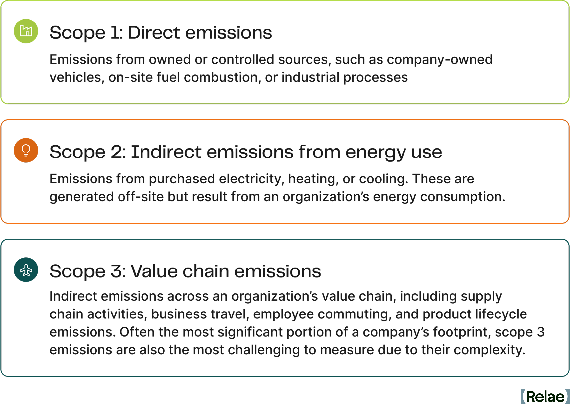
Each scope presents unique challenges and opportunities for reduction. Among them, scope 2 emissions are particularly significant because they stem from purchased energy, which is often generated using fossil fuels. However, numerous reduction mechanisms exist today to help organizations eliminate these emissions, such as improving energy efficiency in order to use less energy, and transitioning to renewable energy sources through market-based mechanisms. Understanding scope 2 emissions is crucial for businesses looking to contribute meaningfully to the global energy transition and achieve sustainability goals.

What Are Scope 2 Emissions?

Scope 2 emissions refer to indirect GHG emissions associated with the consumption of purchased energy. Unlike scope 1 emissions, which result from direct fuel combustion, scope 2 emissions arise from the generation of electricity, steam, heat, or cooling that a company procures from external sources.

The primary sources of scope 2 emissions include:

Purchased electricity: When businesses buy electricity from a utility provider, the emissions from power plants that generate this electricity are classified under scope 2.

Purchased heat, steam, and cooling: Some companies purchase heat, steam, or cooling services instead of generating them on-site. These services often come from centralized facilities that may rely on fossil fuels, thereby contributing to scope 2 emissions.

What sets scope 2 emissions apart from other scopes is the presence of market-based mechanisms that offer multiple pathways for organizations to reduce their carbon footprint. Unlike scope 1, where emissions reductions often require technological shifts or operational changes, scope 2 reductions can be achieved through strategic procurement decisions. The transition to renewable energy sources is an essential component of sustainability strategies, setting the stage for a broader energy transition across industries and economies.

How Are Scope 2 Emissions Measured Today?

The GHG Protocol currently outlines two primary approaches for calculating scope 2 emissions: the location-based method and the market-based method.

Location-Based Method

The location-based method calculates emissions for electricity consumption based on the average emissions intensity of the grid where the energy consumption occurs. This approach is mandatory under various reporting frameworks and does not take into account a company’s procurement choices.

• Relies on grid averages: Emissions are calculated based on regional grid emissions factors rather than specific energy purchases.
• Time-delayed data: Since grid emissions factors are typically updated annually, this method may not reflect real-time energy sourcing changes.
• Limited control: Companies using this method have less direct influence over their reported emissions, as they depend on the overall energy mix of their region.

Market-Based Method

The market-based method, on the other hand, reflects an organization’s actual procurement decisions and energy-sourcing strategies. It accounts for specific contracts, such as power purchase agreements (PPAs), renewable energy credits (RECs), and green tariffs, which allow businesses to claim lower emissions from their purchased electricity.

• Reflects company choices: Emissions calculations take into account contractual agreements for renewable energy purchases.
• Mechanism for electricity transition: Encourages organizations to invest in low-carbon electricity options and actively support the transition to renewables.
• Multiple reduction options: Companies can reduce their scope 2 emissions through a portfolio of mechanisms like PPAs, RECs, and green tariffs, making this method a flexible and strategic tool for decarbonization.

While market-based mechanisms provide flexibility in reducing scope 2 emissions, they also highlight the need for more precise and updated carbon accounting methodologies. For example, some decarbonization strategies, such as time-shifting energy consumption to better match renewable generation, are not accounted for under these methods. This and other limitations mean that the traditional methods outlined in the GHG Protocol are increasingly seen as outdated in an era of rapid changes in energy generation and grid dynamics. As a result, the market is shifting toward more advanced power emission accounting methodologies that provide a more accurate reflection of emissions associated with electricity use.

Proposed Changes to the GHG Protocol Scope 2 Guidance

The current GHG Protocol Scope 2 Guidance provides a market-based instrument methodology, originally designed in the early 2000s, that allows US-based companies to procure renewable energy at any point within a year from anywhere in North America and apply it to any of its annual electricity consumption within that same year. This methodology, as written, allows for a potentially significant mismatch of “emissions caused” (by consuming electricity) versus “emissions avoided” (by generating renewable electricity) in that it does not account for any of the realities of electric grids and generators, which vary significantly over different regions, seasons, and time of day. 

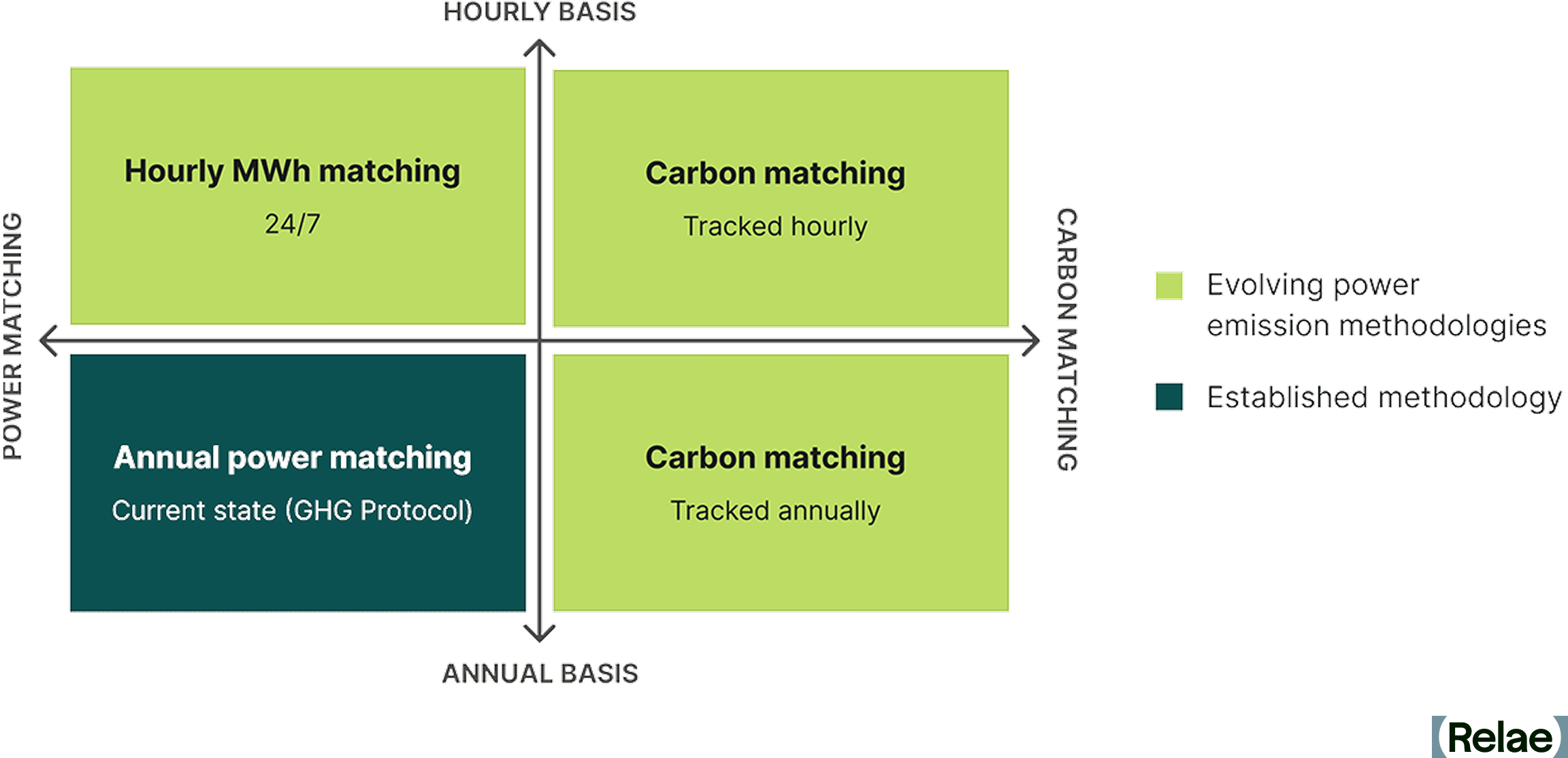
In response to this, the GHG Protocol Scope 2 Guidance is currently undergoing a revision process, which will include how emissions associated with electricity consumption are calculated. A focus of the revision process is on how to better account for the real emissions associated with a corporate’s electricity consumption, and more impactful ways of mitigating them through market-based instruments and other approaches. Advanced power emission accounting methodologies, such as 24/7 power matching and carbon matching, are being explored as ways to better represent the GHG emissions associated with electricity consumption. 

• 24/7 power matching emphasizes matching electricity consumption with an equivalent amount of renewable energy production on an hourly basis.
• Carbon matching emphasizes measuring the emissions impact of incremental electricity consumption or production at a specific time.

These emerging methodologies propose a shift toward more granular temporal and region-specific matching, which could require companies to rethink their emissions reporting approach and explore more advanced tracking tools. They may also introduce new strategies beyond market-based instruments for reducing scope 2 emissions, such as time-shifting energy consumption.

As power grids continue to decarbonize and new digital tools emerge, businesses will need to adapt to these evolving methodologies to remain compliant, enhance sustainability strategies, and achieve meaningful reductions in emissions. Companies that proactively integrate advanced power emission tracking into their carbon accounting strategies will be better positioned to lead in the transition to a low-carbon economy.

How to Reduce Scope 2 Emissions

The GHG Protocol provides multiple mechanisms for reducing scope 2 emissions, allowing organizations to shift their energy consumption toward lower-carbon alternatives. These include:

• Reducing energy consumption: Improving energy efficiency in operations can significantly lower electricity use. In some cases, this involves capital investments in more energy-efficient equipment, but in other cases, it can be based on operational changes such as reducing unnecessary lighting, HVAC, and other services during non-working hours. (Electrification efforts, such as shifting from fossil fuel-powered systems to electric alternatives, may actually increase scope 2 emissions, but this can ultimately reduce overall emissions by correspondingly decreasing scope 1 emissions and allowing for renewable energy procurement.) 
• RECs: Companies can purchase unbundled RECs (emissions “attributes” separated from the actual electricity product) to offset emissions associated with purchased electricity. While there has been criticism of RECs due to their significant range in quality, high-quality RECs are available, which may include ensuring regional matching, financial additionality, on-line date additionality, or tighter temporal generation to consumption matching. The use of high-quality unbundled RECs is the most accessible and realistic option for most smaller-scale companies to address scope 2 emissions. 
• On-site generation and co-location: Installing on-site renewable energy generation, such as solar panels, allows companies to directly offset their electricity consumption from the grid. In some commercial settings, such as companies using leased real estate or co-located data centers, partnering with facilities that prioritize renewable energy procurement can help reduce scope 2 emissions for the facility owner while the facility occupant reduces scope 3 emissions. 
• PPAs: Entering into long-term contracts with renewable energy providers ensures companies receive electricity from clean energy sources while supporting the expansion of renewable generation capacity. PPAs are available with standardized contract terms, and some service providers will aggregate demand from multiple smaller companies to reach the minimum required amount for typical PPA contracts. Hedging products are also available to reduce market risks.
• Green tariffs: Many utilities offer green tariffs that enable businesses to purchase renewable energy directly through their electricity provider, often at a premium but with lower emissions impact. For many smaller companies, this is a more viable approach than a PPA with a single renewable generator.

By adopting a combination of these strategies, businesses can significantly lower their scope 2 emissions while aligning with broader sustainability goals and regulatory requirements. The path to decarbonization requires proactive investment in cleaner energy sources, efficient consumption practices, and leveraging market-based instruments to drive the transition toward a low-carbon future.

Why Does Reducing Scope 2 Emissions Matter?

Reducing scope 2 emissions is the underpinning of decarbonizing the power sector and enabling the global energy transition. In 2025, S&P reported that corporate buyers added 15.2 GW of renewable capacity in the US, up from 9.1 GW in 2024, illustrating the growing impact of the corporate sector on the electricity grid. Cleaner grids translate to lower emissions for all energy users. Organizations that actively reduce their scope 2 emissions can contribute to decreasing demand for fossil fuel-based electricity and accelerate the deployment of renewable energy infrastructure.

For companies that own and operate data centers, this transition is especially important. AI data centers consume large amounts of electricity, and their reliance on purchased power makes them a significant source of scope 2 emissions. Since many businesses rely on third-party data center services, reducing emissions from these facilities also helps lower scope 3 emissions across industries. Corporates can influence data centers by requiring that they have a clear and explicit low-emission power strategy in place before procurement.

Beyond direct corporate benefits, reducing scope 2 emissions has a tangible long-term impact on power grids. Increased investment in renewable energy procurement sends a strong market signal, encouraging utilities and developers to expand clean energy projects. As more companies commit to sourcing renewable energy, the overall mix of grid power shifts, making low-carbon electricity more accessible and reducing reliance on fossil fuel-based generation. Ultimately, widespread corporate action in scope 2 emissions reduction supports the broader decarbonization of power markets and strengthens global climate commitments.

Frequently Asked Questions

Will RECs (renewable energy certificates) still count toward scope 2 reductions under the GHG Protocol's proposed changes?

Under the current Scope 2 Guidance, yes—RECs remain a valid market-based instrument. The proposals from the GHG Protocol's recent consultation range from retaining market-based accounting with stricter quality criteria to restructuring how instrument-based claims are reported altogether, and nothing is final until the revised standard is published. What's clear is that scrutiny is rising, particularly for unbundled RECs with weak temporal or geographic connection to a company's actual consumption, so prioritizing high-quality RECs now is the best way to future-proof a procurement strategy.

How would the proposed hourly and regional matching requirements affect companies that rely on unbundled RECs today?

Hourly (24/7) and regional matching would require renewable generation claims to line up much more closely with when and where a company actually consumes electricity. Companies relying on annually matched, unbundled RECs sourced from distant grids would likely see their reported market-based emissions rise under such requirements. The practical preparation is to start collecting more granular (ideally hourly) consumption data and shift toward RECs and contracts with tighter regional and temporal matching.

What's the practical difference between location-based and market-based scope 2 accounting, and will that distinction survive the GHG Protocol's revision?

The location-based method calculates emissions using the average emissions intensity of the local grid, regardless of procurement choices, while the market-based method reflects a company's actual contracts, such as PPAs, RECs, and green tariffs. The consultation explored options from strengthening the criteria for market-based claims to reporting emissions and market instruments in separate, complementary statements. Both concepts will exist in some form, but companies should expect the requirements behind market-based claims to tighten.

When is the new Scope 2 Guidance expected to take effect, and what should companies do now to prepare?

Per the GHG Protocol's July 2026 development plan, a draft of the revised consolidated Corporate Standard is expected for public consultation in 2027, with a final published standard currently estimated for late 2028, and adoption timelines will follow publication. Companies should take action now. Energy efficiency, PPAs, green tariffs, and high-quality RECs reduce real emissions under any accounting regime. Building hourly consumption tracking and auditing the quality of existing REC portfolios now will make any future transition smoother.

Key Takeaways

• On April 16, 2026, two weeks before the Department of Energy’s (DOE) April 30 deadline for action on the Large Load Proceeding, FERC, the Federal Energy Regulatory Commission, provided a significant update: 
  
  • FERC issued its compliance order on PJM's Bring Your Own Generation (BYOG) tariff; the order approved four interconnection paths, rejected two PJM proposals, and directed PJM to refile by May 18. 
  • FERC's June 2026 order settled a key question around enforcement mechanisms for co-located projects. FERC rejected PJM's Two-Strike proposal (which would have terminated contracts on second violation), allowing only penalties and suspension from the three new transmission services, materially reducing developer downside risk.
  • Notably, BYOG arrangements built on the rejected elements of the compliance filing face restructuring risk before that refile. For deals that clear it, however, energization could begin as early as this summer.
• These proceedings reflect the underlying industry concerns about speed, reliability, and cost equity, shifting the risks and costs of new generation from ratepayers to the large loads, such as data centers, themselves. 
  ‍
• Developers, investors, and project teams can use quantitative grid and load modeling to navigate these risks successfully, converting regulatory exposure into priced engineering decisions.

A New Rulebook for Bring Your Own Generation in PJM

PJM Interconnection (PJM) hosts the highest concentration of data center load growth in the US, managing regional transmission across 13 states in the Eastern US, and commercial operation dates for new generation projects in its current interconnection queue stretch into the early 2030s. Bring Your Own Generation (BYOG) has become the fastest speed-to-power path around that bottleneck. 

BYOG allows large loads, such as data centers, to draw power directly from a co-located generation source connected to the bulk power grid, enabling developers to avoid lengthy interconnection queues and costly transmission upgrades, while drawing limited to no power from the bulk power grid.

The Federal Energy Regulatory Commission’s (FERC) April 16 order is now the rulebook that governs the tariffs that facilitate these BYOG arrangements. Any deal built on the paths FERC closed off must now find a way to align with one of the four approved mechanics before PJM's May 18 compliance refile. Deals that clear the refile could begin to energize as early as this summer.

Below are the top questions the Relae power advisory team is fielding most from hyperscalers, large commercial power buyers, and power producers navigating the mechanics of PJM’s BYOG tariff and the engineering realities of running a co-located project. 

What Is Co-Location?

Co-location refers to a power generation facility sited in close proximity to a large load, such as a data center, that interconnects directly to the bulk power grid. The generator serves that load contractually via a power purchase agreement (PPA), with power flowing through the meter.

BYOG is the predominant co-location model in PJM. Under a typical BYOG arrangement, on-site generation covers the majority of the data center's load (~90%), with only a small residual portion (~10%) supplied from the grid. Each co-located project effectively functions as its own mini-grid, with explicit operational obligations that are less forgiving than standard transmission service (NITS).

Why Did FERC Keep Behind-the-Meter (BTM) and Co-Location Separate?

While BTM and co-location may look similar, they sit in different regulatory buckets. That said, the line between them is less clear-cut than it once was. FERC found existing BTM rules inadequate to address the grid impacts of large co-located loads and directed PJM to treat co-location as a distinct framework. 

At the same time, BTM rules, including how tariffs and distribution charges are applied, remain under revision in a separate PJM proceeding. The two tracks moving in parallel have contributed to the conflation of the frameworks in industry discussion.

How Does Co-Location Differ from BTM Generation?

• Co-location, as this order defines it, is a bulk grid-interconnected arrangement. The host generator remains on the same interstate grid, maintains its interconnection service agreement, and continues exporting power to the grid. The co-located load connects through an approved interconnection mechanic and takes transmission service under a PJM tariff product.
• BTM is a distinct arrangement. The generator sits on the consumer's side of the utility meter and serves the load through a private line, without an interconnection agreement. The load may typically have a grid connection; however, in some circumstances, the generation may be fully off-grid or islanded. By setting a megawatt (MW) threshold for BTM, larger loads with co-located generation may no longer net out their load to reduce transmission and grid charges. FERC's jurisdiction over a BTM arrangement is narrower, and the tariff mechanics that apply to co-location do not apply in the same way.

FERC's rejection of PJM's proposed BTM rule changes illustrates this distinction. The commission is keeping the two categories separate on purpose. Ultimately, FERC’s intention seems to signal that large loads co-located with generation may not be adequately reflected in grid and transmission upgrade costs when these assets are behind the meter. Historically, BTM assets were exempt from these costs because their relatively insignificant power contributions had no meaningful financial impact on the bulk power grid.

That said, the BTM track is still moving. PJM's BTM application rules, including the netting-off mechanism that lets BTM loads avoid utility tariffs, remain under review in parallel proceedings.

For developers, regulatory clarity on co-location and BTM is increasingly critical. In April 2025, FERC upheld its rejection of the Talen-Amazon Susquehanna nuclear BTM interconnection agreement proposal, declining to rehear arguments on the initial decision. To many experts, the split ruling signaled that the structure of PJM’s interconnection service agreement (ISA) is inadequate for large loads operating behind the meter. 

However, in the initial challenge to the Talen-Amazon proposal, utility companies argued that the arrangement would unjustifiably shift transmission costs to other PJM customers. Ultimately, in June 2025, Talen Energy entered into a 1,920 MW, front-of-the-meter power purchase agreement with Amazon Web Services, which does not require FERC’s approval. 

FERC Has Always Regulated Generators, Not Loads. What Changed?

The April 16 order lands inside a larger jurisdictional shift. FERC does not typically regulate load interconnection; its authority sits with the bulk power grid. Under Orders 888 and 2003, FERC has regulated how generators connect to that system (with standardized study deposits, readiness requirements, and withdrawal penalties) while load interconnection has historically been regulated at the distribution level under state jurisdiction.

That generation-only approach to FERC regulation worked for three decades. Now, the scale of AI data centers and other large loads creates interstate impacts that state-level load regulation cannot fully address. Generation co-location breaks the pattern by routing the load through a FERC-regulated generator interconnection agreement rather than a state-regulated load-serving entity, pulling it into federal jurisdiction.

In December 2025, FERC declared PJM's existing interconnection rules (tariff) unjust and unreasonable in the PJM Co-Location Order and directed PJM to revise the tariff. The April 16 order is FERC's review of that rewrite. 

As FERC Commissioner David Rosner wrote in his concurrence to the December 2025 PJM Co-Location Order: "We are trying to meet surging demand while upholding two fundamental values that underpin the electric industry in our country: first, that all customers have a right to receive electric service on a timely basis, and second, that electric service should be reliable and affordable for all customers. Given the scale of new large loads putting demand on our grid today, it is clear that fostering both of these values requires intervention."

Which Four Interconnection Mechanics Did FERC Approve?

The April 16 order (Docket ER26-1088-000, 195 FERC ¶ 61,030) approves four ways for a data center to plug into the PJM grid. Each solves a different bottleneck: available capacity, queue position, study timing, or pre-studied capacity. All four rely on existing PJM and FERC tariff mechanics rather than new constructs, a deliberate choice to reduce legal exposure and speed up adoption. 

1. Sub-full-capacity interconnection service (available capacity). The data center co-locates with an existing host generator, and interconnects at less than the host generator's full capacity, using the portion of the existing interconnection rights the generator does not need.
2. Request acceleration at Decision Points I and II (queue position). Co-located load applications can move ahead of the standard queue at defined checkpoints, subject to PJM's study results. Co-located loads place less demand on the bulk power grid than new large loads without co-located generation, justifying the accelerated treatment. To qualify, projects must demonstrate there will be no significant network updates required or network impact, among other readiness milestones. 
3. Provisional Interconnection Service, or PIS (study timing). Interim interconnection services are provided during the full study, giving developers a bridge to early operations.
4. Surplus Interconnection Service, or SIS (pre-studied capacity). Use of unused capacity at an already-studied generator’s interconnection point, without triggering a new full study.

The four mechanics are different ways of answering the same operational question—how a co-located data center plugs into the grid without triggering a multi-year re-study of the host generator's interconnection—enabling faster speed-to-power.

Which Generators Gain Most From Surplus Interconnection Service?

SIS is the most commercially interesting of the four mechanics for existing generator owners because it monetizes previously stranded capacity.

The generators that benefit most include:

• Retiring or derated thermal units with unused megawatts of interconnection rights at high-value points (for example, retiring coal plants in PJM's eastern and mid-Atlantic footprint).
• Existing nuclear and large thermal plants near concentrated load growth, particularly in Dominion, American Electric Power (AEP), and ComEd territory (the Northern Virginia, Columbus, and Chicago metro zones), where PJM load is most concentrated.
• Storage-paired assets where the underlying generator has capacity headroom that the storage does not fully use (for example, solar-plus-storage or gas-plus-storage sites where the battery sits below the full interconnection rights).

For illustration, a host generator running at roughly 85% of its interconnection rights with a forced outage rate near 5% has material surplus capacity (10%) available to a co-located load, depending on how PJM studies the combined profile.

Owners of underutilized interconnection rights now have an approved tariff path to extract value from them by attracting data centers to co-locate with these generators.

What Transmission Service Does a Co-Located Load Receive?

Connecting to the bulk power grid and taking service from it are two separate decisions. PJM's default transmission service for any load on the system is the Network Integration Transmission Service (NITS), the standard contract for firm power year-round. NITS commits PJM to serve a customer’s full load at any and all times, meaning that PJM may need to wait for generation and/or transmission upgrades before offering it to a large load. 

Recently, PJM reopened its generation interconnection queue after pausing to study its backlog of proposed projects. With 800 proposed projects representing approximately 220 GW in new capacity in 2026, this growth signals progress, but it does not address the underlying permitting and financing challenges that have prevented projects already in the queue from being built.  

The BYOG mechanics are variations that waive or defer parts of NITS for faster speed-to-power. PJM delivers the resulting service through three tariff product types:

1. Firm contract demand: The co-located load holds firm transmission service (consistent with most aspects of NITS) and operates like any other firm load on the system. Availability is site-specific, depending on the point of interconnection. Unlike other NITS customers, entities contracting firm contract demand transmission on behalf of co-located loads cannot exceed the contracted demand level, and loads would be subject to a penalty if they withdraw additional energy beyond the contracted demand capacity. 
2. Non-firm contract demand: The load accepts interruption risk in exchange for faster interconnection or lower-cost service, making it better suited to loads with operational flexibility. It is available at more interconnection points than firm service, but power delivery is subject to curtailment based on real-time grid conditions. This service intends to provide brief and intermittent energy access from the bulk power grid, during available periods, under unanticipated circumstances, such as downtime for the co-located generator. 
3. Interim NITS: A bridge product that provides firm service on an interim basis while the co-located generator is still under construction. The load energizes early; once the generator and any transmission upgrades are complete, the project transitions to a standard NITS arrangement, and the generator can participate in the broader PJM market. However, while the load pays the NITS rate, the load is subject to curtailment under system emergency conditions, posing reliability challenges. 

In practice, a 1,000 MW data center co-located with a 900 MW on-site generator would request 100 MW from PJM under one of these three products.

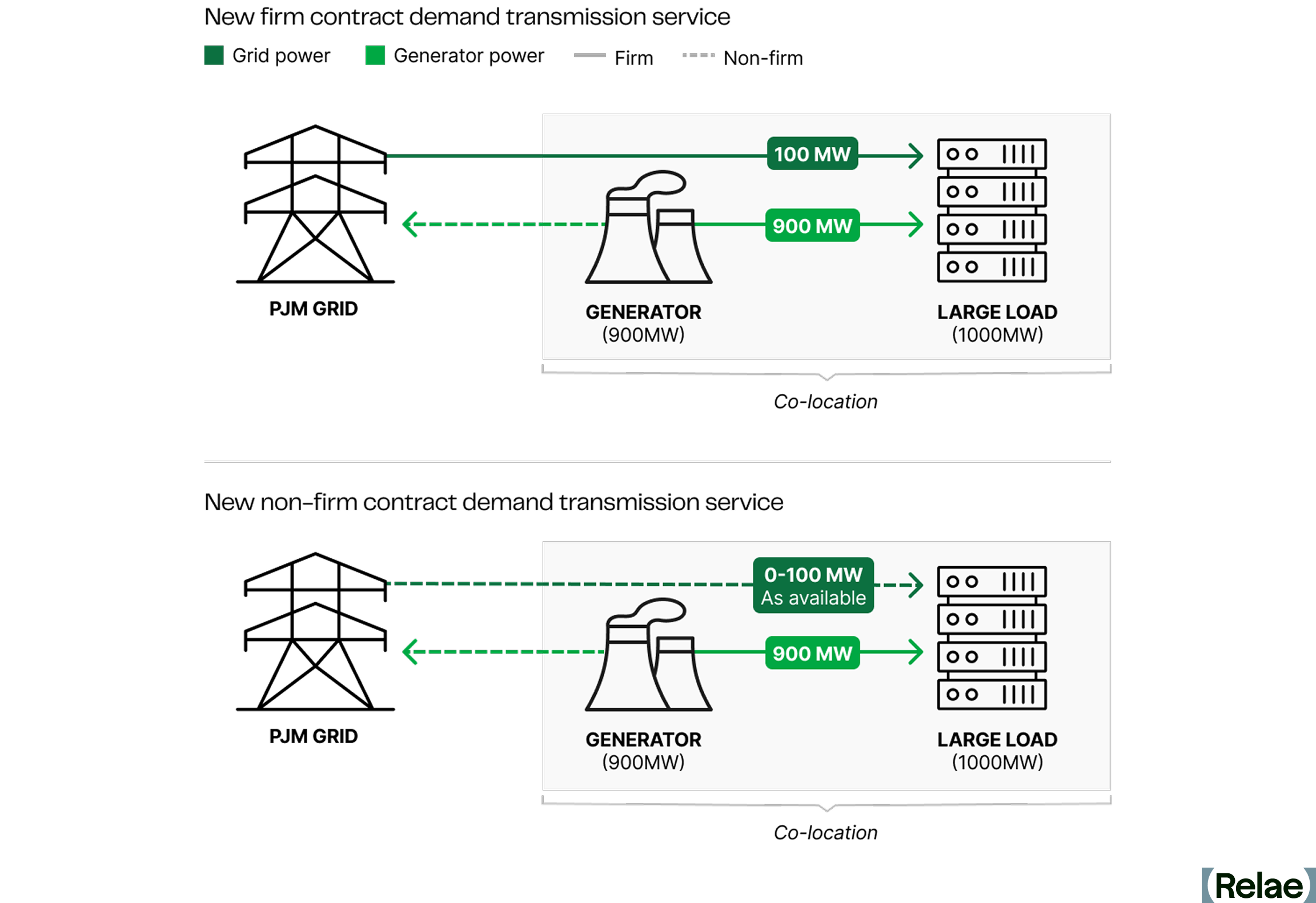
The interconnection mechanic (how the load connects) and the tariff product (what service the load receives) are two distinct decisions. For example, in the case of an interim NITS, a data center and co-located load could connect through a Provisional Interconnection Service (PIS). Other co-located loads may connect by submitting a request for acceleration at Decision Points I and II to secure firm contract demand service. The connection mechanism and tariff will vary based on each co-located load’s unique characteristics and project configuration. 

For clients evaluating specific sites, the right path depends on how much of the host generator's interconnection capacity is available, how sensitive the load is to interruption, and how fast the site needs to energize. Grid modeling allows project teams to quantitatively assess their risk exposure before committing to a tariff product. 

Which Two PJM Proposals Did FERC Reject?

Two elements of PJM's original filing did not make it through the April 16 order.

1. Point of Change in Ownership substitution: PJM proposed swapping in "Point of Change in Ownership" for FERC’s mandated term "Point of Interconnection" in the definition of Co-Located Load. FERC rejected the swap as an unexplained deviation from the Co-Location Order's definition and because it could let transmission owners delay or effectively veto the Point of Change in Ownership location, creating uncertainty for co-located projects.
2. BTM application-rule changes: PJM tried to fold changes to its BTM application rules into this same compliance package. FERC rejected that on the ground the changes did not fall within the scope of the initial order. BTM remains a separate regulatory track; the April 16 order does not settle it.

Project configurations built on either rejected proposal need restructuring before PJM's May 18 refile.

The order also directs PJM to add the PIS definition to the Open Access Transmission Tariff (OATT), Part I, section 1 (paragraph 26), and flags items in paragraph 29, including assessment of the reliability of co-located loads paired with electric storage, as out of scope. 

These determinations should not be seen as FERC rejecting these tariff changes, but rather deeming them outside the scope of the order. They are open questions that belong in a separate docket. The direction to include PIS while declining to address issues not included in the compliance proceeding demonstrates FERC’s focus on speed-to-power, clarifying the rules for new co-located generators to connect to the grid more quickly.  

What Is the Two-Strike Reliability Rule, and Why Does it Matter?

The rules for violating a co-location interconnection service agreement are still being developed, but FERC has urged PJM to issue robust protections to maintain reliability and cost allocation equity. 

For both firm and non-firm contract demand transmission service, PJM will apply a penalty rate to transmission service customers who withdraw more energy from the grid than was contracted. The precise design of these rates for unreserved use is scheduled for a paper hearing this spring; however, developers should cautiously size and appropriately model load and generation sizes, as the penalties for jeopardizing PJM’s reliability are not limited to rates. 

While penalty rate design for unreserved use is underway, PJM proposed a strict Two-Strike reliability rule for co-located projects. If a co-located customer failed to adequately implement automated loadshedding or generator tripping mechanisms during unusual grid conditions, PJM has previewed severe consequences:  

• First strike: a 120-day operational pause for review.
• Second strike: termination of the transmission service contract and return to the NITS interconnection waitlist.

The entire purpose of pursuing a co-located large load configuration is to ensure speed-to-power while maintaining reliability. In a June 2026 order, FERC conceded that there are legitimate reliability concerns with co-located generation misoperation; however, PJM’s proposal to disqualify customers with multiple misoperations is unnecessarily strict. FERC ultimately agreed PJM has the authority to charge penalties to and temporarily suspend services for customers that fail to shed load or curtail, but cannot disqualify customers for misoperation. Data centers will need to rigorously model and design their co-located load and generator facilities with the understanding that multiple reliability violations could strand billion-dollar assets for multiple years. 

Which BYOG Deals Need Restructuring Before the May 18 Refile?

Any deal built around the Point of Change in Ownership substitution or the BTM application-rule changes that FERC rejected needs restructuring. 

In addition, co-located projects that relied on one of the four approved mechanics, but used PJM tariff language from the original December filing, may also need re-papering against the language PJM submits in its forthcoming May 18 compliance filing. Until PJM files that package and FERC accepts it, the operative document is the April 16 order itself.

Counterparties should confirm that operational controls, curtailment rights, and dispute mechanisms in the contract align with the proposed Two-Strike regime and the approved mechanics the project uses.

What Does Grid Modeling Reveal for a Co-Located Project?

Non-firm service is the lowest-cost tariff product for the portion of load the co-located generator does not serve, but availability depends on real-time grid conditions. Grid modeling is how developers size that exposure before signing.

Take the same 1,000 MW data center paired with a 900 MW on-site generator, contracting 100 MW of non-firm service for the residual load. Grid modeling might show non-firm power dropping out in roughly 15% of hours during the summer peak.

If the on-site generator also carries a 5% forced outage rate, the developer faces a meaningful probability of a compound event: grid supply drops out at the same moment the on-site unit trips offline.

In that window, the data center has three options, none of them free: 

1. Curtail load. 
2. Shift the load to another site. 
3. Draw more from the grid than the contract allows, which triggers a Two-Strike violation.

Grid modeling converts that risk into decisions the developer can price. A developer can test whether adding 50 MW of battery storage, contracting 150 MW of firm service instead of 100 MW of non-firm, or adding a smaller backup generator delivers the best risk-adjusted return.

Key Takeaways

• Scope 3.1 emissions, purchased goods and services, can account for up to 67% of a company’s total carbon footprint, making them a critical category for measurement and action.
• Companies can reduce risk, meet stakeholder demands, and strengthen supply chain resilience by proactively managing scope 3.1 emissions.
• Relae empowers organizations to take meaningful action on scope 3.1 through science-based measurement, practical emissions management strategies, and deep supplier engagement.

What Are Scope 3 Emissions and Why Do They Matter?

Scope 3 emissions include all indirect greenhouse gas (GHG) emissions that occur across a company’s value chain. While scope 1 emissions are from directly owned or controlled activities, and scope 2 are indirect emissions from the generation of purchased electricity, heat, or steam, scope 3 emissions encompass upstream and downstream activities throughout the value chain. 

Within scope 3, there are 15 categories, including activities such as raw material extraction, purchased services, shipping, business travel, product use, and end-of-life treatment. Critically, scope 3 emissions usually make up the majority of a company's total carbon footprint. Across sectors, CDP finds supply chain emissions average 26 times a company's operational emissions, and in supply-chain-heavy sectors like apparel, the share exceeds 95%. 

Category 3.1 (purchased goods and services) is often the largest contributor. For many organizations, it can be as much as 67% of their total corporate footprint. Despite being outside a company’s direct operational control, scope 3 emissions are increasingly scrutinized by regulators, investors, and customers alike, making them essential to measure, manage, and reduce. 

What Is Included in Scope 3.1 Emissions?

Scope 3.1 emissions capture all cradle-to-gate emissions associated with products and services procured by an organization. These include emissions from the extraction of raw materials, energy usage, manufacturing processes, waste, and transport and travel up to the point of delivery to the reporting company. As such, the types of activities within this category are quite extensive and disparate. 

Examples of scope 3.1 items include:

• Raw materials (e.g., limestone, copper ore, lumber)
• Intermediate products (e.g., steel, electronic components, platform chemicals)
• Packaging materials
• Office supplies and equipment
• Professional services 
• Cloud computing and software services

The size of scope 3.1 emissions varies widely by industry. For example, a consumer goods manufacturer sourcing large volumes of physical products may see a larger share of emissions in this category than the supplier providing the raw materials. For data centers that run on very low-carbon electricity, equipment and construction can account for 40% of lifetime emissions. For many organizations that are service-based or contract out manufacturing, scope 3.1 can be the most significant emissions category.

What Is the Strategic Value of Scope 3.1?

While scope 3.1 emissions fall outside a company’s direct operational control, they are not beyond its influence. Addressing emissions from purchased goods and services may open up a range of strategic benefits:

• Innovation opportunities through lower-carbon materials and production processes.
• Enhanced supplier relationships and engagement on shared sustainability goals.
• Improved resilience and risk mitigation across supply chains.

By assessing and acting on scope 3.1 emissions, companies can drive meaningful reductions and catalyze change throughout the entire supply chain.

What Are the Methods for Calculating Scope 3.1 Emissions?

There are four methods to calculate scope 3.1 emissions based on the data collected. Each offers a different balance of speed, accuracy, and scalability.

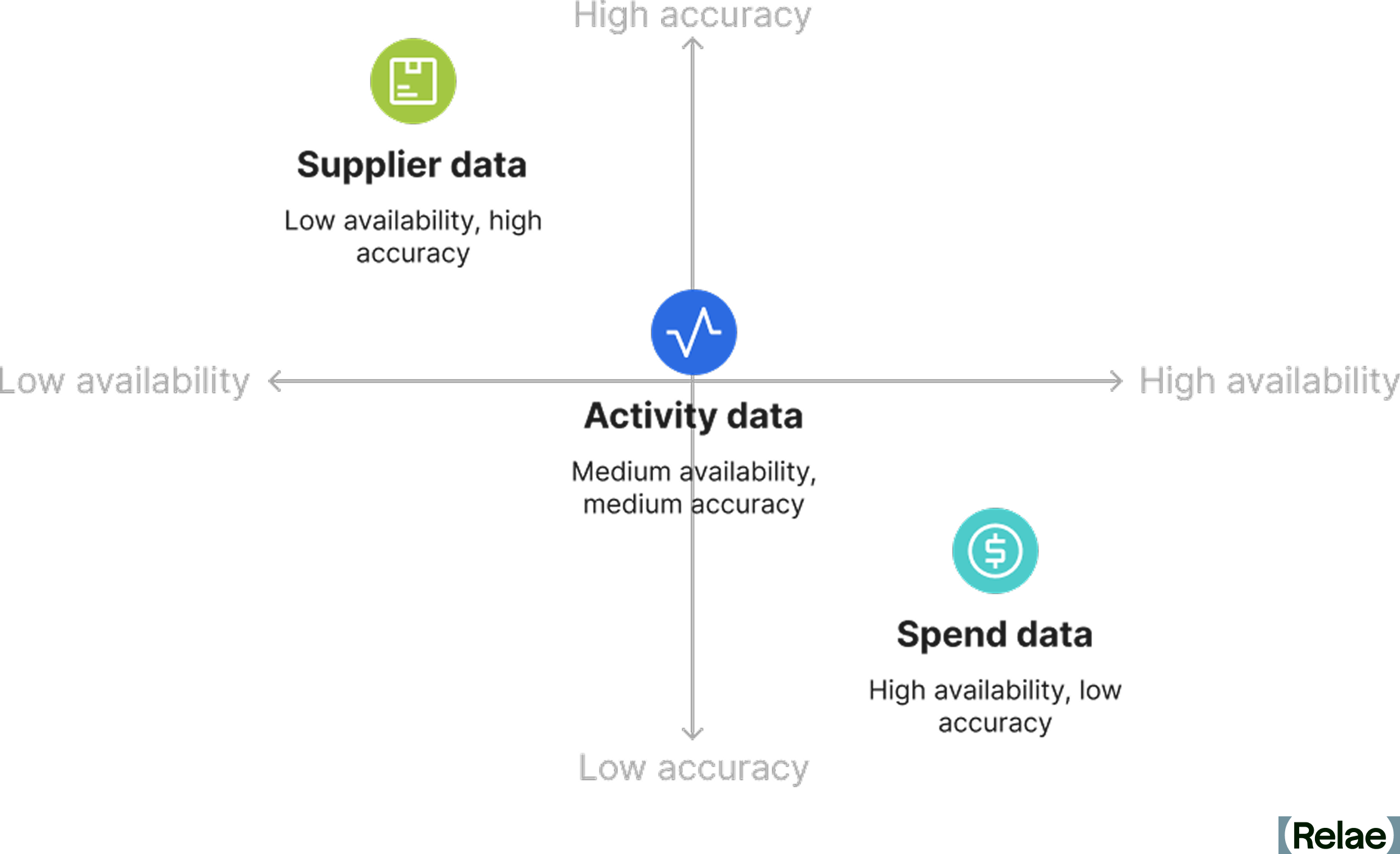
1. The Spend-Based Method

This approach multiplies the amount of money spent on a good or service by an economic emissions factor (e.g., kg CO₂e per dollar spent). Most companies use this approach as a starting point but transition to more accurate methods as they advance in their sustainability journey.

Advantages

• Fast and scalable across categories
• Useful for initial hotspot identification
• Helps fill data gaps when activity data is unavailable

Limitations

• Lower accuracy, especially during periods of inflation or economic volatility
• Cannot reflect actual emissions reductions by suppliers
• Misalignment between price and emissions (e.g., high-cost items may not be high-emission)

2. The Average Data Method

This method uses average emissions factors for goods or services, based on industry datasets. For instance, industry life cycle assessments (LCAs) might be used to estimate the emissions associated with a kilogram of steel purchased.

Advantages

• More accurate than spend-based
• Suitable for companies refining emissions data to enable targeted reductions 

Limitations

• Lack of raw data granularity
• Geographic variation limited

3. The Supplier-Specific Method

The supplier-specific method is the most accurate approach and involves collecting actual emissions data directly from suppliers. This includes LCAs, environmental product disclosures (EPDs), product carbon footprints (PCFs), supplier emissions reports, or Environmental, Social, and Governance (ESG) reports.

Advantages

• High accuracy and granularity
• Builds engagement with suppliers
• Enables tracking of supplier improvements over time

Limitations

• Challenging to scale across many suppliers
• Data may be confidential, inconsistent, or incomplete
• Requires continuous updating of supplier information

4. The Hybrid Approach

Adopting a hybrid approach allows many companies to maximize their data collection efforts by applying the supplier-specific method for high-impact purchases and using average or spend-based methods elsewhere. This tiered approach enables efficient use of resources while maintaining data quality for critical emission sources.

Where Can You Find Scope 3.1 Data?

Data for scope 3.1 emissions typically resides in procurement and finance functions. Purchase orders, invoices, and supplier contracts often contain critical information such as volume, product category, and spend. However, collecting, organizing, and analyzing this data can be resource-intensive, especially for companies with complex and global supply chains. Data type and availability play a key role in determining the method used for calculating emissions, impacting the accuracy and ability to reduce emissions.

What Are the Challenges in Measuring Scope 3.1 Emissions?

As most organizations will attest, measuring scope 3.1 has many challenges, from resource constraints to data availability. As organizations intensify their climate commitments, they are increasingly confronted with a range of technical, logistical, and strategic barriers that make accurate measurement and consistent reporting difficult. Understanding these roadblocks is critical to developing more resilient and impactful scope 3.1 measurement practices. 

• Data availability and quality: Collecting high-quality data is often a bottleneck, with many organizations lacking the systems to track product-level or supplier-specific emissions. Without the proper tracking in place, emissions calculations rely on less accurate methods, making it difficult to reflect or meet reduction efforts.
• Supplier inconsistencies and allocation complexities: Even when suppliers share emissions data, the methodologies, boundaries, and underlying assumptions across them will vary widely. This adds an extra layer of difficulty to data aggregation. Additionally, the allocation of supplier emissions may vary based on the supplier’s chosen method, such as economic (based on spend and supplier revenue/emissions) or service-level (based on units purchased and supplier output/emissions). These inconsistencies can significantly affect reported totals, making it challenging to compare suppliers.
• Complex, multi-tiered supply chains: Upstream emissions can span multiple suppliers across different geographies and industries. Visibility often becomes cloudier beyond Tier 1 suppliers, making it difficult to account for emissions generated deeper in the value chain.
• Timing and synchronization: Aligning procurement, emissions calculation, and reporting cycles can be challenging. Delays in supplier disclosures or emissions factor updates can create reporting lags and misalignment.

Top Five Strategies to Reduce Scope 3.1 Emissions

Reducing scope 3.1 emissions requires balancing precise measurement with targeted action. This means identifying high-impact categories, collaborating with key suppliers, and harnessing available emissions data to improve accuracy and accountability. Here are five strategies organizations can use to start driving impact:

1. Prioritize key categories and suppliers: Not all purchases contribute equally to emissions. Conduct a hotspot analysis to identify the highest-emitting goods or services and prioritize the top suppliers for engagement. Consider prioritizing the share of emissions, the share of procurement spend, and the current methodology type. 
2. Engage suppliers and set expectations: Encourage suppliers to measure and disclose their emissions, invest in LCAs or PCFs, and set their own science-based targets. Collaborative initiatives, such as supplier engagement programs, can support progress.
3. Leverage readily available supplier reports: Many electronic companies, cloud providers, and industrial products provide detailed emissions data through EPDs, LCAs, and specific service emissions reports. For example, AWS and Google offer detailed emissions reports for data hosting and services. Leveraging these can help reduce uncertainty and improve accounting accuracy in software-heavy organizations. However, they should be utilized with caution, as some providers have faced scrutiny in 2026 for reporting efficiency gains without disclosing cloud-specific energy use or the growth in embodied hardware emissions behind it.
4. Identify opportunities for low-carbon inputs: The same reports that help improve reporting accuracy can also provide more detail on the material inputs of purchased goods. This level of information can enable organizations to pursue opportunities for lower-carbon inputs to reduce emissions.
5. Invest in centralized data systems: A centralized platform for carbon accounting data management can streamline emissions tracking, improve visibility, and enable scenario modeling. Several of the other strategies cannot be as effective without the right tools in place to manage this key information. 

Turning Complexity Into Opportunity

Tackling scope 3.1 emissions may feel daunting, but it’s also where some of the biggest climate opportunities lie. By investing in better data, fostering supplier collaboration, and integrating sustainability into procurement practices, companies can unlock innovation, resilience, and long-term value. Organizations that lead on scope 3.1 will not only meet emerging disclosure standards but will shape the low-carbon supply chains of the future.

Frequently Asked Questions

What are scope 3 emissions, and why do they matter?

Scope 3 emissions are all the indirect greenhouse gas emissions in a company's value chain, everything from raw material extraction and purchased services to product use and disposal. They matter because they're usually the majority of a company's footprint. They also fall outside a company’s direct control, which makes them the hardest to measure and the most scrutinized by regulators and investors.

What is included in scope 3.1 emissions?

Scope 3.1 covers the cradle-to-gate emissions of everything a company buys, i.e. all emissions generated up to the point of delivery. That includes raw materials, intermediate goods like steel and electronic components, packaging, office equipment, professional services, and cloud computing. It captures the supplier's extraction, energy use, manufacturing, waste, and transport. It does not include emissions from using or disposing of your own products, which sit in other scope 3 categories.

What are the methods for calculating scope 3.1 emissions?

There are four. The spend-based method multiplies spend by an emissions factor per dollar, which is fast, scalable, and the usual starting point. The average-data method applies industry emissions factors to physical quantities, like kilograms of steel. The supplier-specific method uses actual supplier data such as LCAs, EPDs, or product carbon footprints, and is the most accurate. Most companies land on a hybrid, the final method, which takes supplier-specific data for high-impact purchases and uses estimates elsewhere.

How can companies reduce scope 3.1 emissions?

Start with a hotspot analysis to identify where emissions are coming from. This will usually show that a small share of suppliers and categories drives most of the footprint. From there, engage those suppliers on measurement and targets, use supplier reports and EPDs to replace estimates with real data, and use that detail to identify lower-carbon inputs. Centralized carbon accounting data makes each of these repeatable rather than a one-off exercise.

Do AI data centers' hardware purchases count as scope 3.1 emissions?

Yes, for a data center operator, servers and chips are purchased goods, and therefore count in scope 3.1. 

This article was originally published in collaboration with the Center on Global Energy Policy at Columbia University as part of its Energy Explained series. 

Key Takeaways

• Attention to data centers is skyrocketing in state capitals across the United States.
• In data center bills passed by state legislatures in 2025, two topics dominated: locational incentives (such as reduced sales taxes) and ratepayer protection. Many bills addressing data centers' water use and environmental risks were proposed, but few were enacted.
• Almost all the enacted bills encouraging data centers to locate in a state were passed by Republican legislatures, and more bills addressing data centers' environmental risks were proposed in Democratic legislatures than Republican legislatures. Concern about the impacts of data centers on power prices was bipartisan.

Introduction

From east to west and north to south, in red states and blue states, attention to data centers is skyrocketing in state capitals across the United States. Our research identified more than 190 bills on data centers introduced in state legislatures in the first 11 months of 2025—roughly nine times the number of such bills introduced in 2024. The bills address a wide range of topics, including economic development, ratepayer protection, grid reliability, and disclosure of data centers' energy use and environmental impacts. More than two dozen of these bills were enacted into law.

This newfound interest in data centers in state capitals is unlikely to abate anytime soon. The data center industry is growing at a staggering pace. A recent McKinsey report projected roughly $2.8 trillion in spending on data center infrastructure in the US by 2030. In 2024, data centers used roughly 4–5% of the electricity produced in the United States—a percentage projected to grow sharply in the years ahead. A rapid buildout of data centers and electricity infrastructure to support them offers economic and strategic benefits but also creates risks for ratepayers, water resources and the environment.

State policymakers are on the front lines of these issues. State governments promote economic development, regulate electricity rates and have jurisdiction over many local resource and environmental issues. Different stakeholders have strongly conflicting views on data centers, setting up high-profile debates in state capitals as well as in Washington, DC.

This blog post—the first entry in a project that will explore state data center policies, power prices and related topics—presents these findings.

Methodology: Tracking Data Center Legislation

We (the authors of this article) queried StateNet's database of state legislation to identify bills proposed between January 1 and November 30, 2025 that used several terms including "data center" and "large load." After removing bills that used those terms but addressed different issues, we categorized the remaining bills into topic areas (including tax incentives, ratepayer protection, zoning and siting, disclosure requirements, environmental protections, labor, water resources, clean energy, and research studies) as well as status (enacted, pending, rejected, and passed but vetoed). We supplemented this research with queries to ChatGPT and Gemini to help identify possible gaps in the StateNet review, double-checking links provided by those large language models to ensure the information provided was accurate.

Almost all state legislatures have now adjourned for the year. (Only six state legislatures remain in session in December.) Trends with respect to state legislative activity on data centers in the first 11 months of 2025 included the following.  

Eight Key Data Center Trends From State Legislative Activity in 2025

1. One of the most common objectives of state bills related to data centers was to encourage those facilities to locate in a state.  

• Roughly 50 bills were introduced in state legislatures offering data centers tax incentives or other benefits.  
• Of the more than two dozen bills on data centers enacted by state legislatures, at least nine provided tax incentives or other inducements for siting decisions. Arkansas, Kansas, Kentucky and Minnesota, among other states, all extended or increased sales or use tax exemptions for data centers. Indiana and West Virginia, among others, established favorable zoning and fast-track permitting procedures to facilitate data center construction.

2. State legislatures are paying growing attention to the impact of data centers on power prices. Ratepayer protection and tariff rate issues were among the most popular topics for state legislation on data centers. More than 40 such bills were proposed and at least six such bills passed. Those included:

• Minnesota HF 16, which requires new large grid customers (including data centers), as a group, to cover all their grid costs;
• Texas SB 6, which requires the Texas Public Utility Commission "to support business development in this state while minimizing the potential for stranded infrastructure costs;" and  
• New Jersey A5466 and California SB 57, both of which require the state PUC to study within one year the effect of data centers on electricity costs.

3. Many bills related to the environmental impacts of data centers were introduced in state legislatures, including approximately 30 bills related to water consumption. Only a few of these bills were enacted. Minnesota HF 16, for example, requires close attention to water use in permitting new data centers. Kansas SB 98 makes tax credits for data centers contingent on practices that will "conserve, reuse and replace water."

4. Approximately 40 bills were introduced requiring data centers to disclose their energy use and/or environmental impacts to state authorities, with roughly a dozen bills requiring disclosure to the public. Details regarding metrics and anonymization of reports varied widely. At least three of these disclosure-related bills were enacted, including the following.

• Texas SB 6 requires interconnection applicants to disclose whether they are pursuing other interconnection applications in the state as well as information on onsite back-up generating facilities.
• Minnesota HF 16 requires data centers to disclose information on water consumption volumes.
• Iowa HB 976 requires data centers to submit an annual report to the Department of Revenue detailing the amount of backup power generation fuel and electricity purchased.

5. Several states passed bills limiting tax benefits for data centers.

Iowa limited sales tax exemptions for new data centers to 10 or 15 years (depending on their size), and Florida raised the minimum size for data centers receiving sales tax exemptions from 15 megawatts (MW) to 100 MW.  

6. Texas became the first state in the nation to pass a bill requiring data center operators to enable remote disconnections for use during grid emergencies (referred to as a "kill switch provision").

7. There is little consistency in the legislative text of state bills on data centers.

• Definitions of data centers, thresholds for incentives, and regulations related to disclosure, zoning, siting, environmental impact mitigation and ratepayer protection vary significantly.
• This may be the expected product of variance among state-level policy regimes, and suggests the absence of close coordination among state legislatures or stakeholder groups.

8. The pattern of proposed and enacted bills displayed some partisan patterns.

Almost all the enacted bills encouraging data centers to locate in a state were passed by Republican legislatures. More bills addressing environmental risks from data centers were proposed in Democratic legislatures than Republican legislatures. However bills concerning the impacts of data centers on other ratepayers were enacted in states with Democratic legislatures and governors (including California, New Jersey and Oregon), Republican legislatures and governors (including Texas and Utah) and in which the legislature is controlled by one party and the governor another (including Kansas).

Data centers will be a hot topic as many state legislatures reconvene in January. The Executive Order on state AI laws released by the White House December 11 2025 does not seek to preempt state laws related to data centers (see in particular Section 8b), however questions related to the optimal role of state governments and the federal government on AI and data centers will likely be prominent as well.