From Capture-Ready to Capture-Committed: Decarbonizing Natural Gas with CCS

Key Takeaways

• Scope 2 emissions (indirect emissions from energy use) are increasingly critical to address. With surging electricity demand, especially from data centers, scope 2 is a growing share of corporate emissions and a priority for decarbonization.
• Approaches to scope 2 accounting are evolving—and formal changes are now on the table. Both location-based and market-based methods remain accepted under the Greenhouse Gas Protocol. Still, the Protocol's recently closed public consultation proposes more granular approaches, including 24/7 power and carbon matching, that would better reflect the realities of modern power markets.
• Proven decarbonization levers, such as reducing energy use, entering power purchase agreements, procuring green tariffs, and buying high-quality renewable energy certificates, are already available and impactful. Decarbonization, not just measurement, must be the goal. Companies don’t need to wait to decarbonize. 

Accounting for Indirect Emissions From Energy Use

As businesses and organizations strive to reduce their environmental impact, carbon accounting has become an essential tool for tracking and managing greenhouse gas (GHG) emissions. Carbon accounting helps organizations measure, report, and mitigate their emissions across various activities. A key framework for categorizing these emissions is the Greenhouse Gas Protocol (GHG Protocol), which classifies emissions into three scopes:

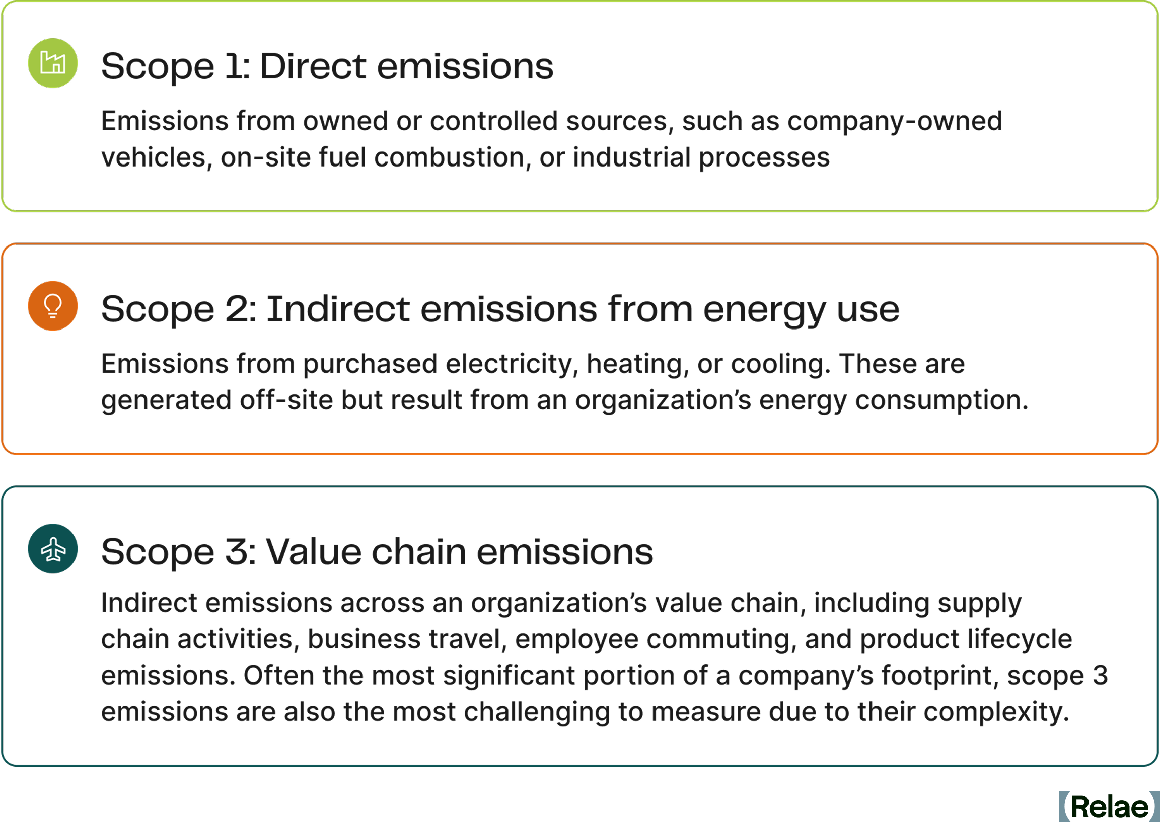
Each scope presents unique challenges and opportunities for reduction. Among them, scope 2 emissions are particularly significant because they stem from purchased energy, which is often generated using fossil fuels. However, numerous reduction mechanisms exist today to help organizations eliminate these emissions, such as improving energy efficiency in order to use less energy, and transitioning to renewable energy sources through market-based mechanisms. Understanding scope 2 emissions is crucial for businesses looking to contribute meaningfully to the global energy transition and achieve sustainability goals.

What Are Scope 2 Emissions?

Scope 2 emissions refer to indirect GHG emissions associated with the consumption of purchased energy. Unlike scope 1 emissions, which result from direct fuel combustion, scope 2 emissions arise from the generation of electricity, steam, heat, or cooling that a company procures from external sources.

The primary sources of scope 2 emissions include:

Purchased electricity: When businesses buy electricity from a utility provider, the emissions from power plants that generate this electricity are classified under scope 2.

Purchased heat, steam, and cooling: Some companies purchase heat, steam, or cooling services instead of generating them on-site. These services often come from centralized facilities that may rely on fossil fuels, thereby contributing to scope 2 emissions.

What sets scope 2 emissions apart from other scopes is the presence of market-based mechanisms that offer multiple pathways for organizations to reduce their carbon footprint. Unlike scope 1, where emissions reductions often require technological shifts or operational changes, scope 2 reductions can be achieved through strategic procurement decisions. The transition to renewable energy sources is an essential component of sustainability strategies, setting the stage for a broader energy transition across industries and economies.

How Are Scope 2 Emissions Measured Today?

The GHG Protocol currently outlines two primary approaches for calculating scope 2 emissions: the location-based method and the market-based method.

Location-Based Method

The location-based method calculates emissions for electricity consumption based on the average emissions intensity of the grid where the energy consumption occurs. This approach is mandatory under various reporting frameworks and does not take into account a company’s procurement choices.

• Relies on grid averages: Emissions are calculated based on regional grid emissions factors rather than specific energy purchases.
• Time-delayed data: Since grid emissions factors are typically updated annually, this method may not reflect real-time energy sourcing changes.
• Limited control: Companies using this method have less direct influence over their reported emissions, as they depend on the overall energy mix of their region.

Market-Based Method

The market-based method, on the other hand, reflects an organization’s actual procurement decisions and energy-sourcing strategies. It accounts for specific contracts, such as power purchase agreements (PPAs), renewable energy credits (RECs), and green tariffs, which allow businesses to claim lower emissions from their purchased electricity.

• Reflects company choices: Emissions calculations take into account contractual agreements for renewable energy purchases.
• Mechanism for electricity transition: Encourages organizations to invest in low-carbon electricity options and actively support the transition to renewables.
• Multiple reduction options: Companies can reduce their scope 2 emissions through a portfolio of mechanisms like PPAs, RECs, and green tariffs, making this method a flexible and strategic tool for decarbonization.

While market-based mechanisms provide flexibility in reducing scope 2 emissions, they also highlight the need for more precise and updated carbon accounting methodologies. For example, some decarbonization strategies, such as time-shifting energy consumption to better match renewable generation, are not accounted for under these methods. This and other limitations mean that the traditional methods outlined in the GHG Protocol are increasingly seen as outdated in an era of rapid changes in energy generation and grid dynamics. As a result, the market is shifting toward more advanced power emission accounting methodologies that provide a more accurate reflection of emissions associated with electricity use.

Proposed Changes to the GHG Protocol Scope 2 Guidance

The current GHG Protocol Scope 2 Guidance provides a market-based instrument methodology, originally designed in the early 2000s, that allows US-based companies to procure renewable energy at any point within a year from anywhere in North America and apply it to any of its annual electricity consumption within that same year. This methodology, as written, allows for a potentially significant mismatch of “emissions caused” (by consuming electricity) versus “emissions avoided” (by generating renewable electricity) in that it does not account for any of the realities of electric grids and generators, which vary significantly over different regions, seasons, and time of day. 

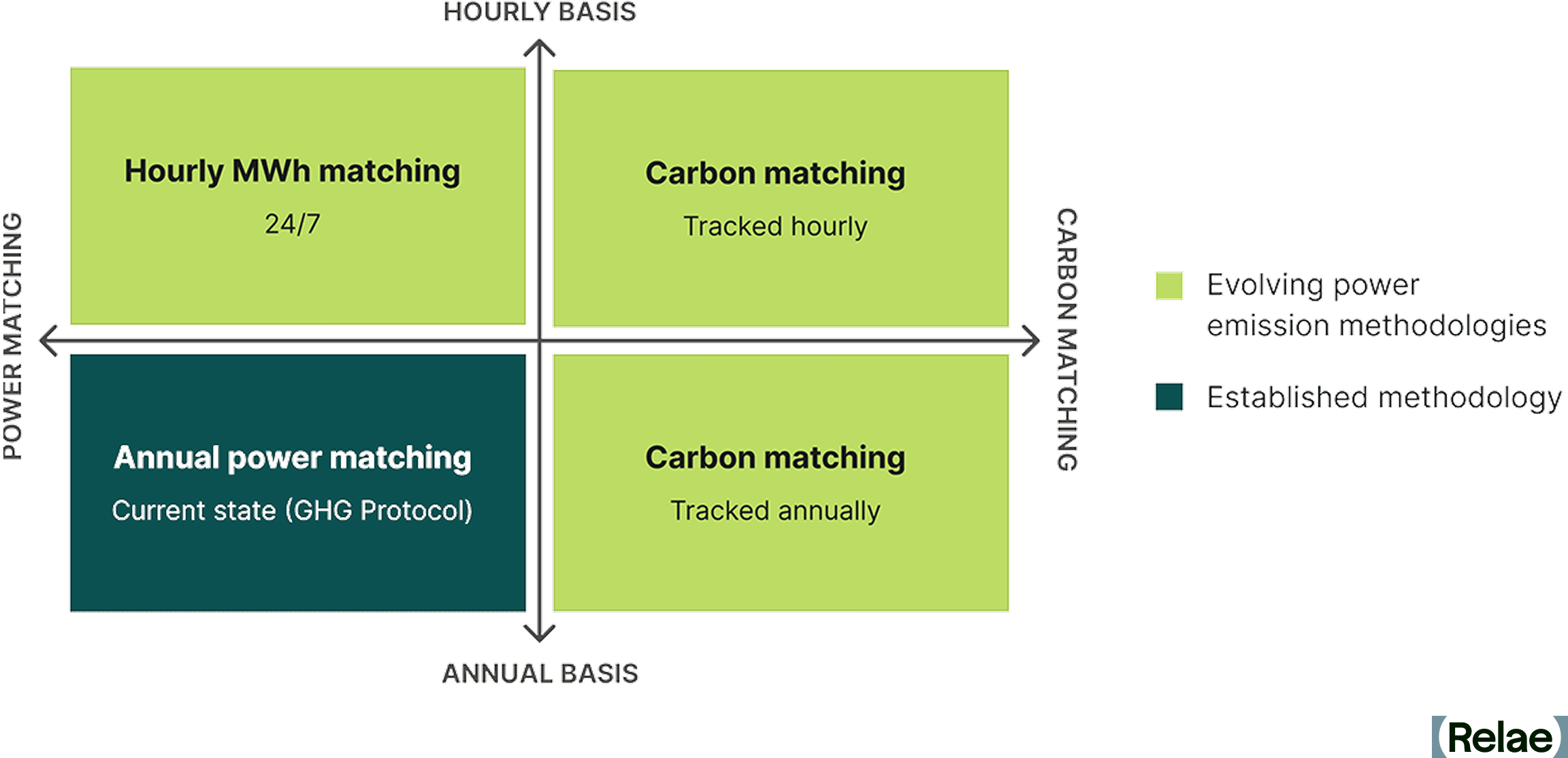
In response to this, the GHG Protocol Scope 2 Guidance is currently undergoing a revision process, which will include how emissions associated with electricity consumption are calculated. A focus of the revision process is on how to better account for the real emissions associated with a corporate’s electricity consumption, and more impactful ways of mitigating them through market-based instruments and other approaches. Advanced power emission accounting methodologies, such as 24/7 power matching and carbon matching, are being explored as ways to better represent the GHG emissions associated with electricity consumption. 

• 24/7 power matching emphasizes matching electricity consumption with an equivalent amount of renewable energy production on an hourly basis.
• Carbon matching emphasizes measuring the emissions impact of incremental electricity consumption or production at a specific time.

These emerging methodologies propose a shift toward more granular temporal and region-specific matching, which could require companies to rethink their emissions reporting approach and explore more advanced tracking tools. They may also introduce new strategies beyond market-based instruments for reducing scope 2 emissions, such as time-shifting energy consumption.

As power grids continue to decarbonize and new digital tools emerge, businesses will need to adapt to these evolving methodologies to remain compliant, enhance sustainability strategies, and achieve meaningful reductions in emissions. Companies that proactively integrate advanced power emission tracking into their carbon accounting strategies will be better positioned to lead in the transition to a low-carbon economy.

How to Reduce Scope 2 Emissions

The GHG Protocol provides multiple mechanisms for reducing scope 2 emissions, allowing organizations to shift their energy consumption toward lower-carbon alternatives. These include:

• Reducing energy consumption: Improving energy efficiency in operations can significantly lower electricity use. In some cases, this involves capital investments in more energy-efficient equipment, but in other cases, it can be based on operational changes such as reducing unnecessary lighting, HVAC, and other services during non-working hours. (Electrification efforts, such as shifting from fossil fuel-powered systems to electric alternatives, may actually increase scope 2 emissions, but this can ultimately reduce overall emissions by correspondingly decreasing scope 1 emissions and allowing for renewable energy procurement.) 
• RECs: Companies can purchase unbundled RECs (emissions “attributes” separated from the actual electricity product) to offset emissions associated with purchased electricity. While there has been criticism of RECs due to their significant range in quality, high-quality RECs are available, which may include ensuring regional matching, financial additionality, on-line date additionality, or tighter temporal generation to consumption matching. The use of high-quality unbundled RECs is the most accessible and realistic option for most smaller-scale companies to address scope 2 emissions. 
• On-site generation and co-location: Installing on-site renewable energy generation, such as solar panels, allows companies to directly offset their electricity consumption from the grid. In some commercial settings, such as companies using leased real estate or co-located data centers, partnering with facilities that prioritize renewable energy procurement can help reduce scope 2 emissions for the facility owner while the facility occupant reduces scope 3 emissions. 
• PPAs: Entering into long-term contracts with renewable energy providers ensures companies receive electricity from clean energy sources while supporting the expansion of renewable generation capacity. PPAs are available with standardized contract terms, and some service providers will aggregate demand from multiple smaller companies to reach the minimum required amount for typical PPA contracts. Hedging products are also available to reduce market risks.
• Green tariffs: Many utilities offer green tariffs that enable businesses to purchase renewable energy directly through their electricity provider, often at a premium but with lower emissions impact. For many smaller companies, this is a more viable approach than a PPA with a single renewable generator.

By adopting a combination of these strategies, businesses can significantly lower their scope 2 emissions while aligning with broader sustainability goals and regulatory requirements. The path to decarbonization requires proactive investment in cleaner energy sources, efficient consumption practices, and leveraging market-based instruments to drive the transition toward a low-carbon future.

Why Does Reducing Scope 2 Emissions Matter?

Reducing scope 2 emissions is the underpinning of decarbonizing the power sector and enabling the global energy transition. In 2025, S&P reported that corporate buyers added 15.2 GW of renewable capacity in the US, up from 9.1 GW in 2024, illustrating the growing impact of the corporate sector on the electricity grid. Cleaner grids translate to lower emissions for all energy users. Organizations that actively reduce their scope 2 emissions can contribute to decreasing demand for fossil fuel-based electricity and accelerate the deployment of renewable energy infrastructure.

For companies that own and operate data centers, this transition is especially important. AI data centers consume large amounts of electricity, and their reliance on purchased power makes them a significant source of scope 2 emissions. Since many businesses rely on third-party data center services, reducing emissions from these facilities also helps lower scope 3 emissions across industries. Corporates can influence data centers by requiring that they have a clear and explicit low-emission power strategy in place before procurement.

Beyond direct corporate benefits, reducing scope 2 emissions has a tangible long-term impact on power grids. Increased investment in renewable energy procurement sends a strong market signal, encouraging utilities and developers to expand clean energy projects. As more companies commit to sourcing renewable energy, the overall mix of grid power shifts, making low-carbon electricity more accessible and reducing reliance on fossil fuel-based generation. Ultimately, widespread corporate action in scope 2 emissions reduction supports the broader decarbonization of power markets and strengthens global climate commitments.

Frequently Asked Questions

Will RECs (renewable energy certificates) still count toward scope 2 reductions under the GHG Protocol's proposed changes?

Under the current Scope 2 Guidance, yes—RECs remain a valid market-based instrument. The proposals from the GHG Protocol's recent consultation range from retaining market-based accounting with stricter quality criteria to restructuring how instrument-based claims are reported altogether, and nothing is final until the revised standard is published. What's clear is that scrutiny is rising, particularly for unbundled RECs with weak temporal or geographic connection to a company's actual consumption, so prioritizing high-quality RECs now is the best way to future-proof a procurement strategy.

How would the proposed hourly and regional matching requirements affect companies that rely on unbundled RECs today?

Hourly (24/7) and regional matching would require renewable generation claims to line up much more closely with when and where a company actually consumes electricity. Companies relying on annually matched, unbundled RECs sourced from distant grids would likely see their reported market-based emissions rise under such requirements. The practical preparation is to start collecting more granular (ideally hourly) consumption data and shift toward RECs and contracts with tighter regional and temporal matching.

What's the practical difference between location-based and market-based scope 2 accounting, and will that distinction survive the GHG Protocol's revision?

The location-based method calculates emissions using the average emissions intensity of the local grid, regardless of procurement choices, while the market-based method reflects a company's actual contracts, such as PPAs, RECs, and green tariffs. The consultation explored options from strengthening the criteria for market-based claims to reporting emissions and market instruments in separate, complementary statements. Both concepts will exist in some form, but companies should expect the requirements behind market-based claims to tighten.

When is the new Scope 2 Guidance expected to take effect, and what should companies do now to prepare?

Per the GHG Protocol's July 2026 development plan, a draft of the revised consolidated Corporate Standard is expected for public consultation in 2027, with a final published standard currently estimated for late 2028, and adoption timelines will follow publication. Companies should take action now. Energy efficiency, PPAs, green tariffs, and high-quality RECs reduce real emissions under any accounting regime. Building hourly consumption tracking and auditing the quality of existing REC portfolios now will make any future transition smoother.

The AI and Climate Execution Challenge

Data center energy capacity in the US is projected to increase from 25 GW to 120 GW by 2030—a fivefold increase. Hyperscalers are projected to invest $7 trillion globally in data center infrastructure through 2030, with approximately $2.8 trillion invested in the US. 

While 2025 was defined by a 'scale at all costs' scramble for compute, in 2026, the new mandate is responsible scale: reconciling voracious power demands with aggressive net-zero commitments and rising energy costs. 

Grid constraints determine the geography and velocity of growth, forcing companies into complex trade-offs between speed-to-market and “clean, firm” power, which can take years to develop. Evolving carbon accounting rules are shifting procurement strategies and infrastructure choices at this trillion-dollar scale, creating a “carbon debt”—embodied emissions that will stay on the books for decades. In 2026, the competitive advantage likely belongs to those who integrate power, hardware, and climate strategy from day one. 

Powering AI: Grid Reliability, Constraints, and Interconnection

Grid infrastructure faces reliability challenges from aging systems and capacity constraints.  Interconnection queues stretch three to five years for renewables, while large electrical load interconnection lacks consistent standards.

Federal Regulatory Response

The federal government is moving to standardize these processes, with a critical decision point in 2026. For companies planning data center deployments in 2026, understanding these regulatory shifts is likely essential to realistic timeline and site selection planning.

On October 30, 2025, the US Department of Energy (DOE) leveraged Section 403(a) of the DOE Organization Act to direct the Federal Energy Regulatory Commission (FERC) to issue a rulemaking to “ensure efficient, timely, and non-discriminatory load interconnections” for large (>20 MW) electrical loads. 

By April 30, 2026, FERC is expected to issue a final rule on large electrical load interconnections for grid operators, providing federal regulations for approval pathways,  timelines, and rates. 

Public comments on DOE’s advanced notice of proposed rulemaking were due on December 5, 2025, and grid operators, utilities, NGOs, and customers submitted over 150 comments reflecting a wide range of perspectives. 

While federal standardization should reduce procedural uncertainty, it doesn't create new grid capacity. Even with clearer approval pathways, the underlying supply-demand mismatch remains a primary gating factor for growth.

Bridging the Supply-Demand Gap

Data center energy demand is surging, but new clean electricity generation takes years to build. This mismatch between accelerating demand and slow-building supply is forcing the industry to pursue solutions on two timelines: near-term load flexibility strategies that unlock existing capacity, and long-term generation investments that build new power supply.

Load Flexibility: Near-Term Grid Access

Load flexibility is emerging as a possible path to faster grid connection. Oracle, NVIDIA, Emerald AI, and Salt River Project's joint research demonstrated 25% power reduction during peak hours through workload tiering. The demonstration shows that if data centers reduce consumption during peak times (roughly 1% of the year), it unlocks 126 GW of currently constrained capacity that could be available now.

Large power loads increasingly face incentives or mandates to demonstrate flexibility as part of interconnection agreements, making this an access requirement, not an optional efficiency measure. For example, Senate Bill 6 in Texas mandates that data centers and other large loads must reduce their consumption during certain grid peak times. Many other state legislatures are passing legislation that will impact data centers.

Storage has shifted from smoothing renewables to enabling multiple strategies: making intermittent renewables firmer, providing grid reliability services, and supporting 24/7 matching. Storage may emerge as a solution to allow data centers to reduce grid consumption during peak hours while maintaining operations.

Relae helps clients design load flexibility strategies under evolving regulatory frameworks: evaluating behind-the-meter generation options, sizing storage for peak reduction scenarios, and structuring interconnection configurations that preserve optionality across accounting methodologies.

Clean Firm Power: Long-Term Generation

Hyperscalers remain committed to clean, firm generation that’s reliable: power that's both low-carbon and dispatchable 24/7. Natural gas with carbon capture and storage (CCS) is emerging as a critical bridge technology. Google's 400 MW CCS power agreement with Broadwing, expected online in 2029, demonstrates commercial demand at scale. 

In our analysis evaluating CCS pathways, commercial viability depends on rigorous assessment of permitting timelines, capital and operating costs, storage geology, vendor compatibility, and 45Q tax credit optimization. Execution has been most prevalent where technology intersects with regulatory approval and storage access.

Hyperscalers are also investing across geothermal, nuclear, including Small Modular Reactors (SMR), hydrogen, and fusion. Long-duration energy storage has also been an area of focus. Each has different risk profiles and opportunities across technical maturity, permitting, commercial viability, emission accounting methodology, dispatchability, and political support. 

Evaluating these pathways requires multi-dimensional frameworks. Each technology faces distinct challenges: SMRs struggle with execution complexity, geothermal with extended development periods, and hydrogen with production-dependent carbon intensity. Tax credit eligibility (particularly 45Q for CCS and 45V for hydrogen) significantly impacts project economics.

Both power generation and data center Infrastructure site selection require integrating environmental and social vulnerability data to avoid community conflicts that delay or stop projects.

Power Accounting Rules Determine Clean Energy Procurement

The Greenhouse Gas (GHG) Protocol extended the public consultation period for proposed scope 2 guidance changes to January 31, 2026. The results will determine clean energy procurement strategies and the carbon value of load flexibility for the next decade.

The proposed shift in electricity emissions accounting could increase clean energy procurement costs for buyers. The accounting methodological debates matter for hyperscalers: 24×7 energy matching versus carbon matching. The issues of deliverability (being located in the same grid region) and additionality (being new, rather than repurposed, generation) are also hotly debated.

These different frameworks strongly influence whether natural gas with CCS, nuclear, geothermal, or battery-backed renewables are considered optimal for a site, and whether load flexibility has carbon value.

Companies need to model scenarios across advanced power emissions methodologies, evaluating portfolio costs and carbon performance before final standards are published in 2027. Companies are also signing forward renewable energy certificate contracts (RECs) and structuring power purchase agreements (PPAs) now to preserve optionality across scenarios.

AI Infrastructure Emissions at Scale

Data center construction creates substantial scope 3 emissions, and their relative importance depends on grid carbon intensity. For facilities powered by average-carbon grids, scope 2 operational emissions dominate. But for data centers powered by very low-carbon electricity (renewables or nuclear), scope 3 embodied emissions can represent 40% of total lifetime greenhouse gas emissions.

In AI data centers, IT equipment drives the majority of embodied emissions. Chips and memory account for 67%, followed by structural materials at 17%, with server power supplies, aluminum, and other components comprising the final 16%. 

Direct procurement of low-carbon materials faces constraints: limited supply, geographic concentration, and contracting complexity. Environmental Attribute Credits (EACs) provide an interim pathway by decoupling environmental benefits from physical materials, but require rigorous quality standards and verification to ensure real emissions reductions.

Our high-quality EAC criteria, developed with Microsoft, establish standards that separate market-making from greenwashing. Levelized Cost of Carbon Abatement frameworks make materials decisions comparable to power decisions, treating infrastructure decarbonization as portfolio optimization, not separate workstreams.

Carbon Removal: Addressing Residual Emissions

Complete supply chain decarbonization by 2030 isn't feasible. Despite aggressive efforts to procure clean power and reduce construction emissions, residual emissions will remain significant. For hyperscalers with net-zero commitments, carbon dioxide removal (CDR) has shifted from an optional component to a structural necessity. Microsoft remains the world's largest CDR buyer, and Google increased purchases 14-fold from 2023 to 2024.

CDR credit quality varies widely. Companies must apply science-based principles to evaluate credits. Our Criteria for High-Quality CDR, developed in collaboration with Microsoft, establishes six science-based principles for evaluating credits—critical as emerging hyperscaler and other corporate demand high-integrity supply.

AI and Climate: Looking Ahead

The window for strategic maneuvering is narrow. The AI infrastructure buildout is happening now, and the decisions made in 2026 will impact a company’s cost structure and carbon profile for years. 

Companies treating power, infrastructure, and decarbonization as separate workstreams will face compounding constraints. The winners of the AI era will be those who integrate power, infrastructure, and carbon strategy into a single, cohesive system. 

Key Takeaways

• Power demand is outrunning buildout. Meeting large load growth requires more than new generation; it requires faster interconnection and congestion relief on existing transmission lines. 
• Dynamic line rating (DLR) is available today, deploys in months, and enables faster speed-to-power. On the right thermally congested lines, DLR can unlock more capacity at a fraction of new infrastructure cost. In one utility demonstration, 5% to 10% of additional capacity was enough to clear most of the congestion on the lines studied.
• DLR has been held back by weak incentives, but that is changing. Utilities earn a regulated return on capital they invest in new assets, which favors building new infrastructure over lower-cost solutions like DLR. Load growth and new Federal Energy Regulatory Commission (FERC) mandates are starting to shift the calculus.

The Grid Cannot Expand Fast Enough for AI Demand, But It Can Carry More

Power demand is booming as data centers scale across the US grid, and current grid infrastructure cannot supply it. This constraint is physical, not financial. Meeting this demand requires a significant amount of power generation and infrastructure upgrades. More than 2 terawatts of generation and storage sit in interconnection queues, roughly 1.5x the total installed generation capacity in the US. 

Regional markets are working to accelerate generation buildouts, but connecting that generation to the transmission network remains expensive and slow to match speed-to-power needs. New high-voltage lines take years to permit, cost between $2 million and $6 million per mile to build, and major projects routinely take five to ten years from identification to energization. For example, PJM Interconnection LLC (PJM) identified the Doubs–Goose Creek 500 kilovolt (kV) corridor as a bottleneck feeding Data Center Alley in 2023 and set June 2027 as the date a fix was needed. Dominion Energy's published schedule for its portion of that rebuild anticipates a completion date of 2031.

A number of studies^1,2 show there is headroom in the bulk transmission system. Grid-enhancing technologies, such as dynamic line rating (DLR), can convert part of that headroom into capacity today while new generation and transmission are being built. DLR lets suitable transmission lines increase their carrying capacity in real time, unlocking that headroom at a fraction of the cost of a buildout. Realizing that value is a targeting exercise with a key question: On which thermally limited lines can DLR actually relieve congestion? 

What Is Dynamic Line Rating?

Dynamic line rating is a method for calculating a transmission line's real-time carrying capacity using live weather and conductor-temperature data. It lets grid operators safely carry more power whenever weather conditions allow.

Most transmission lines operate under a static rating: a fixed, conservative limit on current, set for worst-case weather and held all year. The limit is based on temperature, because pushing too much current can overheat the conductor wire. Metal conductors expand as they heat, which can make them sag and touch trees or other obstacles, causing short circuits or fires. Real conditions almost always cool a conductor better than the worst-case assumption a static rating is built on. That means the line can carry more current while staying at the same maximum conductor temperature, and therefore within the same sag and clearance envelope. That headroom is exactly what DLR captures: instead of leaving it on the table, DLR recalculates the line's rating in real time so operators can use the extra capacity safely.

Beyond a static rating is the ambient-adjusted rating (AAR), which many utilities have begun adopting. An AAR recalculates the rating from forecast ambient air temperature, typically hourly and out to several days. DLR goes further, adding wind speed and direction, solar heating, and in some deployments the conductor's measured temperature.

DLR technologies rest on a heat-balance algorithm: how fast a line heats up (from electric current and sunshine) versus how fast it cools off (from wind and cold air). The calculations are standardized in IEEE 738 in North America and CIGRE 601 internationally. The data feeding those calculations can come from line-mounted sensors, weather models, or both, depending on a tradeoff between per-span accuracy and the cost of installing sensors along every span.

Even so, DLR remains limited in the US, and AAR has been slow to arrive. FERC's Order 881 required the transmission providers it regulates to adopt AAR by July 2025, but FERC has granted numerous extensions. PJM became the first to fully implement AAR in March 2026, while Midcontinent Independent System Operator (MISO) and New York Independent System Operator (NYISO) are not expected until 2028.

The Near-Term Value of DLR: Reducing Grid Congestion

DLR's value is immediate. It can be installed in months, not years, so a currently congested line can start carrying more power the moment conditions allow, reducing congestion right away. When cheaper generation is available upstream of that line, DLR cuts costs directly, because grid operators no longer need to dispatch pricier generation downstream of the congestion to supply load. That means DLR can reduce congestion costs in the current delivery year, compared to a transmission line rebuild that sits in a decade-long queue. 

Over a longer horizon, utility planners can build that headroom into long-term capacity models. This is important, because current capacity-expansion and integrated resource plan (IRP) models still run on static or seasonal ratings, and typically leave out the potential gains from grid-enhancing technologies like DLR. 

NERC's large loads white paper and FERC's RM26-4 rulemaking both raise the issue of how utilities can absorb multi-hundred-megawatt data center requests without a decade-long transmission build. Solutions like DLR are one of the few tools that can compress that timeline. 

The hardware itself is cheap: sensors and data management cost a small fraction of any physical upgrade. That means the economics comes down to identifying the lines that benefit most from DLR. This is particularly important because on most US grids, congestion concentrates on a small number of lines that repeatedly reach their limits. On those lines, DLR can cut congestion costs directly and defer costlier upgrades, while its potential on other lines may be far lower. As a result, identifying those high-potential, thermally congested lines is essential.

Proven DLR Examples in the Industry 

Real deployments show DLR can reduce a meaningful share of transmission congestion costs, with extra carrying capacity above the static rating running roughly 5% to 30%, depending on how often that capacity is available. In Oncor's ERCOT demonstration, 5% of additional capacity would have relieved up to 60% of congestion on the target lines, and 10% would have practically eliminated it. PPL Electric in Pennsylvania/PJM reports annual customer savings of $23 million after deploying DLR across its initial three lines. The DLR installation cost about $250,000, against a rebuild alternative that would have cost about $50 million and taken far longer. 

The contrast abroad is instructive. Austria's grid operator, APG, recorded about $13 million a year in congestion savings across roughly 15% of its network. While these savings are real, it's important to recognize that these results come from single, well-chosen, badly congested lines. 

The UK's National Grid began with a two-year DLR trial on a single 275 kV circuit in 2022, expanded to more than 275 kilometers of its network by 2025, with estimated consumer savings of about $26 million a year. In April 2026, National Grid signed a five-year contract covering 585 kilometers more, with most installations due by 2028 and potential savings of up to $66 million. Each expansion followed measured results from the stage before it.

Where the Headroom Is: Screening PJM's Data Center Alley

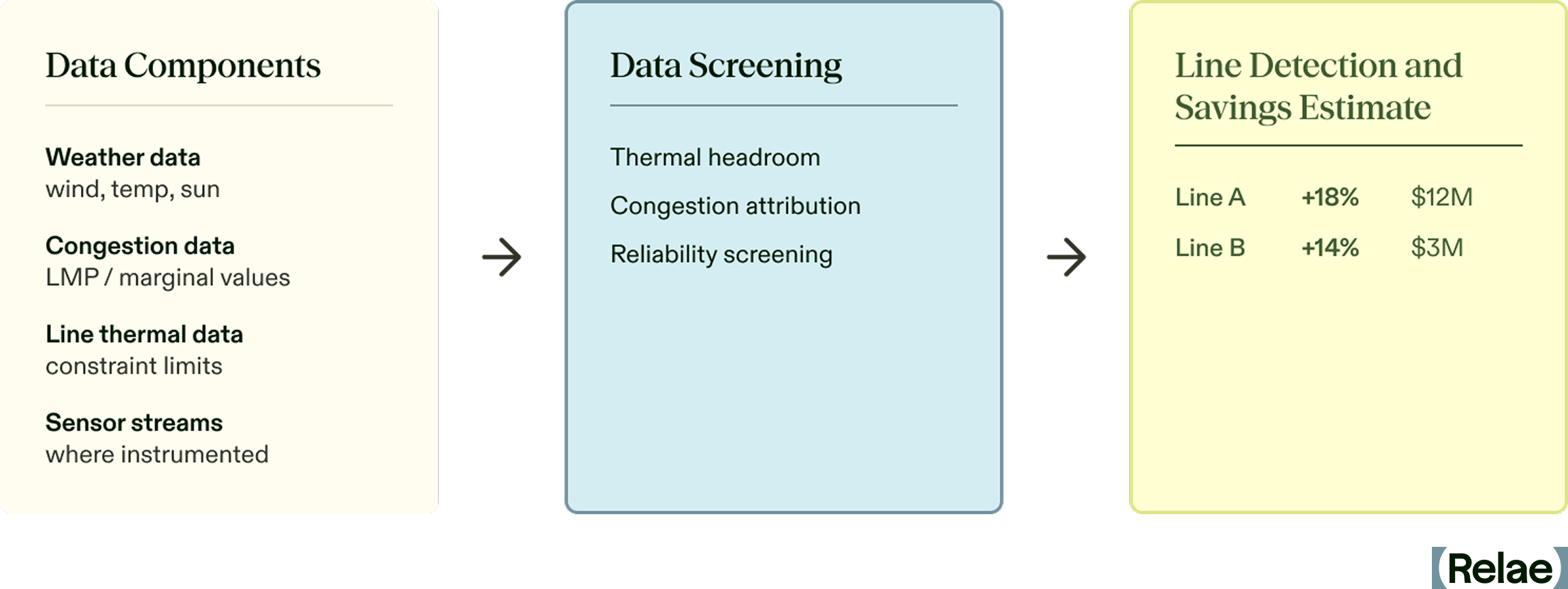
To illustrate the congestion savings from DLR, Relae screened PJM's five-minute real-time market record for every binding transmission constraint in 2025. For each one, we captured the shadow price, the marginal value of relaxing that constraint.³

Our analysis focused on thermal constraints, and then identified lines that bind frequently, in conditions milder than the worst case their static rating was set for, which is when a conductor's true rating sits above its static assumption. For the lines that we identified, congestion costs were added over the binding hours to set a bound on the savings that could result from DLR. That full amount would not necessarily be realized in practice, because the shadow price values only the next megawatt freed, and relieving one line can shift the constraint to the next. However, it serves as a useful estimate for the scale of savings that could be achieved.

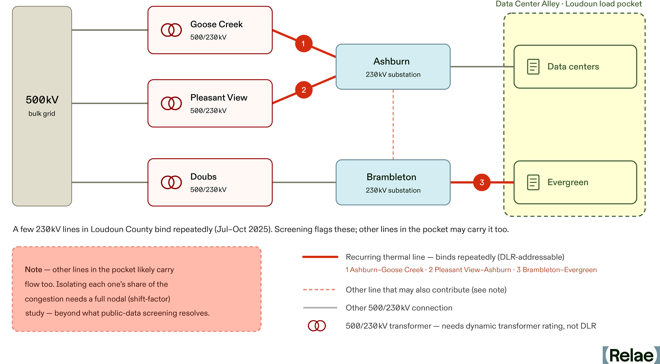
We ran the analysis on the Dominion (DOM) zone in PJM, home to Data Center Alley in Loudoun County, Virginia. Figure 2 shows a high-level section of the grid. The 500 kV bulk grid steps down through transformers to the 230 kV substations feeding the data centers, with the lines that experience recurring congestion highlighted. A handful of those 230 kV lines showed up as binding thermal constraints again and again. 

The congestion in DOM isn't constant, and it concentrates in particular months and within the day in particular hours. Figure 3 shows three transmission lines within the DOM zone and the number of hours each was thermally congested in each hour-of-day slot over 2025. Binding concentrates in the warm months and, within the day, from late morning through early evening. 

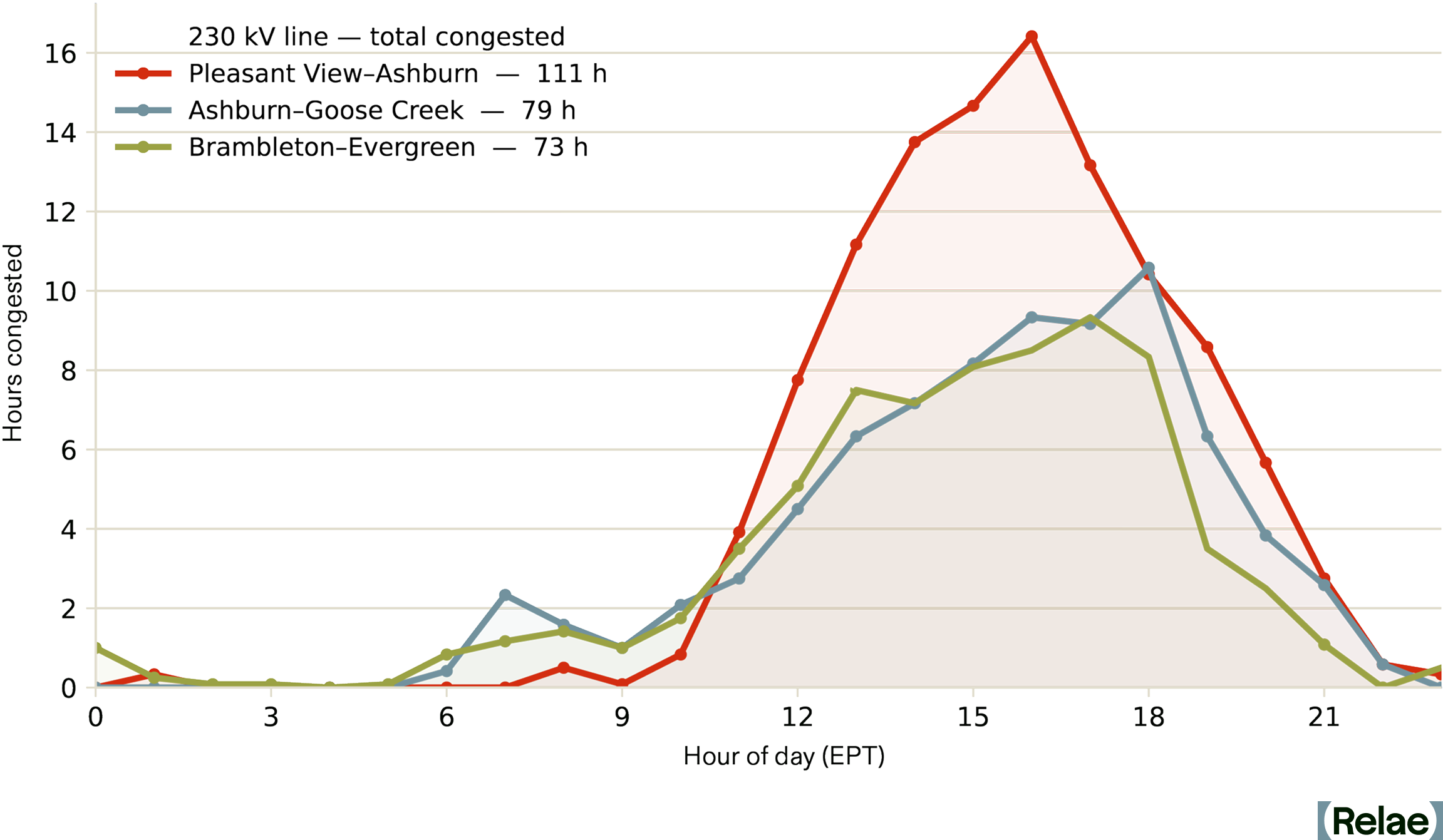
At first glance, this period looks like the wrong window for DLR. The local weather record says otherwise. These periods turn out to be some of the windiest hours of the day, not the stillest. Median wind speed at Dulles ran about 3.5 m/s, above the 0.6 m/s crossflow a static rating conventionally assumes, with fewer than 5% of observations falling below that threshold. Median ambient temperature in those hours was about 26°C, against the 35–40°C a static summer rating is typically built for. Across all three lines, the large majority of congested hours coincided with weather that would have supported a materially higher rating. 

Valuing just one megawatt of DLR relief at each five-minute shadow price, the estimated savings are worth roughly $300,000 in this three-line example across about 263 line-hours.⁴

Because the value concentrates on a handful of thermally limited, heavily congested lines, and because the operational case has to be made line by line, capturing the opportunity is fundamentally an analytics problem: find the right lines, and prove the savings.

What Does It Take to Scale DLR?

DLR is cheap and effective, but two things stand between it and broader adoption: incentives and advanced grid analytics.

The utility cost-of-service model recovers investment in generation and transmission assets and earns its profit as a regulated return on the capital deployed. Because rates recover capital rather than power delivered, utilities have a stronger incentive to build or upgrade lines than to move more power across the ones they already own. That bias toward capital investment over optimization is why a mature technology has stayed niche in the US for years. Regulators have started to look more closely at this, but the main federal rule still mandates the milder AAR, not DLR, and leaves the return model untouched.

Contingency analysis compounds the problem. Current models are built around fixed line limits. A rating that changes hour to hour adds real modeling work, and more importantly, the system still has to hold under worst-case contingencies. So while operators already forecast weather daily for wind and solar, the harder step is trusting a forecast enough to commit a transmission limit against it. That takes significant predictive analytics built into system planning, not bolted on after.⁵

How Policy Is Starting to Shift the Calculus

Policy is starting to move the incentive problem. FERC's Order 881 made AAR the minimum for the transmission providers it regulates (effective July 2025, with several operators on extended timelines) and required markets to be capable of accepting dynamic ratings. PJM has started to implement this: PPL Electric has run sensor-based DLR on nine congested lines since 2022, feeding PJM's day-ahead markets. 

Order 1920, FERC's first long-term transmission-planning overhaul in more than a decade, now requires planners to formally evaluate grid-enhancing technologies like DLR against conventional builds. It stops short of mandating deployment, but it forces a comparison utilities used to skip. That comparison is now written into filed tariff processes (PJM filed its plan in December 2025). Those first cycles only began in 2026, and the order allows up to three years to reach a selection, so the results are still pending. 

A shared-savings incentive, letting a utility keep a slice of the congestion savings it creates, has been proposed to FERC and championed in the Advancing GETs Act, but it isn't yet a rule, so the core misalignment stands. DOE's GRIP program has funded grid-enhancing deployments, and by early 2026, 16 states had some form of advanced transmission technology requirement, with Colorado adding its Grid Optimization Act in April 2026.

The newest pressure is coming from the demand side. Through 2025–26, FERC began overhauling how large loads connect to the grid, and while none of it touches the utility's return on capital, it changes who sees the costs. FERC issued show-cause orders directing all six grid operators to justify or reform their large-load rules. This tees up consideration of alternative transmission technologies in study processes and greater transparency into costs. 

And the rules are moving toward making the large load pay for the upgrades its connection requires. Pennsylvania's model large-load tariff, for example, recommends utilities charge data centers for the upgrades their interconnection makes necessary. It also instructs utilities to let those customers self-construct certain upgrades, including some affecting the wider grid. That combination is what matters. The party paying the bill now has a reason to ask whether a cheaper fix exists and, in at least one state, a route to build it. We have not yet seen a DLR deployment selected this way, because these frameworks are only months old, but the cost gap between a DLR fix and a rebuild is becoming visible to the party who pays the difference.

How Relae Helps Find the Value of DLR  

Through our Power, Data, and Innovation practice, Relae combines transmission congestion data, line-level thermal constraints, and short-term weather forecasts into a single view of where dynamic ratings would actually pay. The output is a short list of candidate lines, each with a modeled capacity uplift and an estimated dollar value, turning a vague “DLR is promising” into a priced, line-by-line decision. It is the transmission-side complement to our work on the interconnection queue and demand-side flexibility. All three are ways of closing the gap between demand and delivered capacity faster than new construction allows.

Key Takeaways

• Larger power users are securing behind-the-meter (BTM) power to bypass grid constraints, pairing data centers with third-party-owned generation assets that deliver electricity through a private line rather than the grid.
• BTM power arrangements can create confusion about electricity emissions classification: the power users neither own the generating asset nor purchase electricity from the grid, leading some to misclassify those emissions as scope 3 in their corporate GHG inventories. But the GHG Protocol's Corporate Standard is clear: BTM electricity emissions belong in scope 2.
• Misclassifying BTM emissions can create reputational and regulatory risk. Relae can help organizations get this right before the contract closes.

Why Large Power Users Are Turning to Behind-the-Meter Power

Large power users are consuming more electricity due to data center growth and are looking to add capacity faster than the grid can support, which is having a direct impact on corporate emissions. For example, between 2020 and 2024, Microsoft’s location-based scope 2 emissions rose 130%, and Google’s rose 92%, driven almost entirely by soaring electricity demand from AI infrastructure. 

To bypass grid congestion and long interconnection queues, many are turning to behind-the-meter (BTM) power. It’s a pragmatic solution to a real supply problem, but it’s opening an urgent carbon accounting question: when the BTM asset is owned and operated by a third party, where should we account for those emissions?

There has been some confusion that has resulted in companies pursuing an interpretation that would place those emissions in scope 3. The GHG Protocol’s Corporate Standard says otherwise, and the stakes of getting this wrong are high.

What Is Behind-the-Meter Power Generation?

Behind-the-meter refers to electricity generated on the power consumer’s side of the utility meter, bypassing the grid, and typically located on or near the site where the power is consumed. 

In most BTM arrangements for a data center, a third-party developer builds and operates a generation asset, such as natural gas, geothermal, or renewable energy, and delivers electricity directly to the facility through a private transmission line. There is no utility meter, no grid connection, and no standard energy invoice. 

This structure allows companies to access large, reliable blocks of power without waiting years for grid interconnection approvals. Since the company does not own or operate the generation asset and is not purchasing electricity through a conventional utility relationship, this arrangement has created some uncertainty around how to account for the associated emissions. 

Can BTM Electricity Emissions Be Classified As Scope 3?

In this scenario, no. The GHG Protocol's Corporate Standard is unambiguous: BTM electricity emissions belong in scope 2, not scope 3. Yet, some companies have been confused about this classification.

There is broad agreement that since the power users do not own or operate the generating asset, those emissions do not belong in scope 1. Divergence starts when we consider that the company is purchasing BTM power, i.e., not from the grid. Since no electricity is acquired from the grid, some argue that rather than accounting for these emissions in scope 2, they are better placed in scope 3, category 8: emissions from leased assets. 

The appeal is obvious for BTM power consumers. Scope 3 emissions face less scrutiny from investors, auditors, and regulators who focus most of their attention on scopes 1 and 2. Classifying BTM emissions as scope 3 would reduce near-term pressure to act. However, the GHG Protocol is unambiguous in its stance.

What the GHG Protocol Actually Says

The GHG Protocol’s Scope 2 Guidance states that “organizations must quantify emissions from the generation of acquired and consumed electricity, steam, heat, or cooling (collectively referred to as ‘electricity’).” The method of delivery, whether grid or BTM, does not change the classification. 

If a company consumes electricity from a BTM source, the emissions from generating that electricity belong in scope 2. Section 5.4 of the Scope 2 Guidance addresses BTM power generation directly: “the company with operational or financial control of the energy generation facility reports those emissions in scope 1, following the operational control approach, while the consumer of the energy reports the emissions in scope 2.”

This resolves the question completely. The emissions sit in scope 1 if the company has operational or financial control of the asset, or in scope 2 if a third party controls it.

The GHG Protocol’s Corporate Value Chain (Scope 3) Accounting and Reporting Standard reinforces this conclusion. “Category 8 includes emissions from the operation of assets that are leased by the reporting company in the reporting year and not already included in the reporting company’s scope 1 or scope 2 inventories.”

Because BTM electricity emissions are captured by the Scope 2 Guidance, the scope 3 category 8 does not apply.

Get the Accounting Right Before the Contract Closes

The GHG Protocol is unambiguous: behind-the-meter electricity emissions belong in scope 2 for companies that consume, but do not control the generating asset. This means that BTM contract terms are crucial to determining how the emissions will be classified, since the GHG Protocol assigns scope based on who holds operational or financial control of the generating asset. 

Companies that move fast on BTM capacity without understanding this distinction risk locking in a scope 1 or scope 2 obligation they didn't anticipate or building a reporting strategy around a scope 3 interpretation the GHG Protocol doesn't support. This can become a reputational or even a regulatory liability that is far harder to address after the contract is signed.

[cta]

Key Takeaways

• On April 16, 2026, two weeks before the Department of Energy’s (DOE) April 30 deadline for action on the Large Load Proceeding, FERC, the Federal Energy Regulatory Commission, provided a significant update: 
  
  • FERC issued its compliance order on PJM's Bring Your Own Generation (BYOG) tariff; the order approved four interconnection paths, rejected two PJM proposals, and directed PJM to refile by May 18. 
  • FERC's June 2026 order settled a key question around enforcement mechanisms for co-located projects. FERC rejected PJM's Two-Strike proposal (which would have terminated contracts on second violation), allowing only penalties and suspension from the three new transmission services, materially reducing developer downside risk.
  • Notably, BYOG arrangements built on the rejected elements of the compliance filing face restructuring risk before that refile. For deals that clear it, however, energization could begin as early as this summer.
• These proceedings reflect the underlying industry concerns about speed, reliability, and cost equity, shifting the risks and costs of new generation from ratepayers to the large loads, such as data centers, themselves. 
  ‍
• Developers, investors, and project teams can use quantitative grid and load modeling to navigate these risks successfully, converting regulatory exposure into priced engineering decisions.

A New Rulebook for Bring Your Own Generation in PJM

PJM Interconnection (PJM) hosts the highest concentration of data center load growth in the US, managing regional transmission across 13 states in the Eastern US, and commercial operation dates for new generation projects in its current interconnection queue stretch into the early 2030s. Bring Your Own Generation (BYOG) has become the fastest speed-to-power path around that bottleneck. 

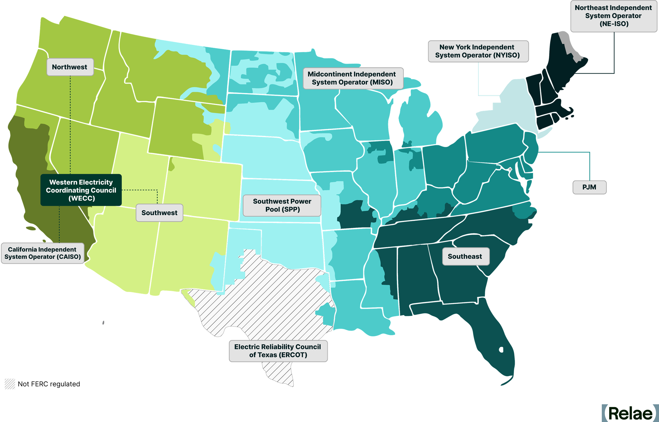
BYOG allows large loads, such as data centers, to draw power directly from a co-located generation source connected to the bulk power grid, enabling developers to avoid lengthy interconnection queues and costly transmission upgrades, while drawing limited to no power from the bulk power grid.

The Federal Energy Regulatory Commission’s (FERC) April 16 order is now the rulebook that governs the tariffs that facilitate these BYOG arrangements. Any deal built on the paths FERC closed off must now find a way to align with one of the four approved mechanics before PJM's May 18 compliance refile. Deals that clear the refile could begin to energize as early as this summer.

Below are the top questions the Relae power advisory team is fielding most from hyperscalers, large commercial power buyers, and power producers navigating the mechanics of PJM’s BYOG tariff and the engineering realities of running a co-located project. 

What Is Co-Location?

Co-location refers to a power generation facility sited in close proximity to a large load, such as a data center, that interconnects directly to the bulk power grid. The generator serves that load contractually via a power purchase agreement (PPA), with power flowing through the meter.

BYOG is the predominant co-location model in PJM. Under a typical BYOG arrangement, on-site generation covers the majority of the data center's load (~90%), with only a small residual portion (~10%) supplied from the grid. Each co-located project effectively functions as its own mini-grid, with explicit operational obligations that are less forgiving than standard transmission service (NITS).

Why Did FERC Keep Behind-the-Meter (BTM) and Co-Location Separate?

While BTM and co-location may look similar, they sit in different regulatory buckets. That said, the line between them is less clear-cut than it once was. FERC found existing BTM rules inadequate to address the grid impacts of large co-located loads and directed PJM to treat co-location as a distinct framework. 

At the same time, BTM rules, including how tariffs and distribution charges are applied, remain under revision in a separate PJM proceeding. The two tracks moving in parallel have contributed to the conflation of the frameworks in industry discussion.

How Does Co-Location Differ from BTM Generation?

• Co-location, as this order defines it, is a bulk grid-interconnected arrangement. The host generator remains on the same interstate grid, maintains its interconnection service agreement, and continues exporting power to the grid. The co-located load connects through an approved interconnection mechanic and takes transmission service under a PJM tariff product.
• BTM is a distinct arrangement. The generator sits on the consumer's side of the utility meter and serves the load through a private line, without an interconnection agreement. The load may typically have a grid connection; however, in some circumstances, the generation may be fully off-grid or islanded. By setting a megawatt (MW) threshold for BTM, larger loads with co-located generation may no longer net out their load to reduce transmission and grid charges. FERC's jurisdiction over a BTM arrangement is narrower, and the tariff mechanics that apply to co-location do not apply in the same way.

FERC's rejection of PJM's proposed BTM rule changes illustrates this distinction. The commission is keeping the two categories separate on purpose. Ultimately, FERC’s intention seems to signal that large loads co-located with generation may not be adequately reflected in grid and transmission upgrade costs when these assets are behind the meter. Historically, BTM assets were exempt from these costs because their relatively insignificant power contributions had no meaningful financial impact on the bulk power grid.

That said, the BTM track is still moving. PJM's BTM application rules, including the netting-off mechanism that lets BTM loads avoid utility tariffs, remain under review in parallel proceedings.

For developers, regulatory clarity on co-location and BTM is increasingly critical. In April 2025, FERC upheld its rejection of the Talen-Amazon Susquehanna nuclear BTM interconnection agreement proposal, declining to rehear arguments on the initial decision. To many experts, the split ruling signaled that the structure of PJM’s interconnection service agreement (ISA) is inadequate for large loads operating behind the meter. 

However, in the initial challenge to the Talen-Amazon proposal, utility companies argued that the arrangement would unjustifiably shift transmission costs to other PJM customers. Ultimately, in June 2025, Talen Energy entered into a 1,920 MW, front-of-the-meter power purchase agreement with Amazon Web Services, which does not require FERC’s approval. 

FERC Has Always Regulated Generators, Not Loads. What Changed?

The April 16 order lands inside a larger jurisdictional shift. FERC does not typically regulate load interconnection; its authority sits with the bulk power grid. Under Orders 888 and 2003, FERC has regulated how generators connect to that system (with standardized study deposits, readiness requirements, and withdrawal penalties) while load interconnection has historically been regulated at the distribution level under state jurisdiction.

That generation-only approach to FERC regulation worked for three decades. Now, the scale of AI data centers and other large loads creates interstate impacts that state-level load regulation cannot fully address. Generation co-location breaks the pattern by routing the load through a FERC-regulated generator interconnection agreement rather than a state-regulated load-serving entity, pulling it into federal jurisdiction.

In December 2025, FERC declared PJM's existing interconnection rules (tariff) unjust and unreasonable in the PJM Co-Location Order and directed PJM to revise the tariff. The April 16 order is FERC's review of that rewrite. 

As FERC Commissioner David Rosner wrote in his concurrence to the December 2025 PJM Co-Location Order: "We are trying to meet surging demand while upholding two fundamental values that underpin the electric industry in our country: first, that all customers have a right to receive electric service on a timely basis, and second, that electric service should be reliable and affordable for all customers. Given the scale of new large loads putting demand on our grid today, it is clear that fostering both of these values requires intervention."

Which Four Interconnection Mechanics Did FERC Approve?

The April 16 order (Docket ER26-1088-000, 195 FERC ¶ 61,030) approves four ways for a data center to plug into the PJM grid. Each solves a different bottleneck: available capacity, queue position, study timing, or pre-studied capacity. All four rely on existing PJM and FERC tariff mechanics rather than new constructs, a deliberate choice to reduce legal exposure and speed up adoption. 

1. Sub-full-capacity interconnection service (available capacity). The data center co-locates with an existing host generator, and interconnects at less than the host generator's full capacity, using the portion of the existing interconnection rights the generator does not need.
2. Request acceleration at Decision Points I and II (queue position). Co-located load applications can move ahead of the standard queue at defined checkpoints, subject to PJM's study results. Co-located loads place less demand on the bulk power grid than new large loads without co-located generation, justifying the accelerated treatment. To qualify, projects must demonstrate there will be no significant network updates required or network impact, among other readiness milestones. 
3. Provisional Interconnection Service, or PIS (study timing). Interim interconnection services are provided during the full study, giving developers a bridge to early operations.
4. Surplus Interconnection Service, or SIS (pre-studied capacity). Use of unused capacity at an already-studied generator’s interconnection point, without triggering a new full study.

The four mechanics are different ways of answering the same operational question—how a co-located data center plugs into the grid without triggering a multi-year re-study of the host generator's interconnection—enabling faster speed-to-power.

Which Generators Gain Most From Surplus Interconnection Service?

SIS is the most commercially interesting of the four mechanics for existing generator owners because it monetizes previously stranded capacity.

The generators that benefit most include:

• Retiring or derated thermal units with unused megawatts of interconnection rights at high-value points (for example, retiring coal plants in PJM's eastern and mid-Atlantic footprint).
• Existing nuclear and large thermal plants near concentrated load growth, particularly in Dominion, American Electric Power (AEP), and ComEd territory (the Northern Virginia, Columbus, and Chicago metro zones), where PJM load is most concentrated.
• Storage-paired assets where the underlying generator has capacity headroom that the storage does not fully use (for example, solar-plus-storage or gas-plus-storage sites where the battery sits below the full interconnection rights).

For illustration, a host generator running at roughly 85% of its interconnection rights with a forced outage rate near 5% has material surplus capacity (10%) available to a co-located load, depending on how PJM studies the combined profile.

Owners of underutilized interconnection rights now have an approved tariff path to extract value from them by attracting data centers to co-locate with these generators.

What Transmission Service Does a Co-Located Load Receive?

Connecting to the bulk power grid and taking service from it are two separate decisions. PJM's default transmission service for any load on the system is the Network Integration Transmission Service (NITS), the standard contract for firm power year-round. NITS commits PJM to serve a customer’s full load at any and all times, meaning that PJM may need to wait for generation and/or transmission upgrades before offering it to a large load. 

Recently, PJM reopened its generation interconnection queue after pausing to study its backlog of proposed projects. With 800 proposed projects representing approximately 220 GW in new capacity in 2026, this growth signals progress, but it does not address the underlying permitting and financing challenges that have prevented projects already in the queue from being built.  

The BYOG mechanics are variations that waive or defer parts of NITS for faster speed-to-power. PJM delivers the resulting service through three tariff product types:

1. Firm contract demand: The co-located load holds firm transmission service (consistent with most aspects of NITS) and operates like any other firm load on the system. Availability is site-specific, depending on the point of interconnection. Unlike other NITS customers, entities contracting firm contract demand transmission on behalf of co-located loads cannot exceed the contracted demand level, and loads would be subject to a penalty if they withdraw additional energy beyond the contracted demand capacity. 
2. Non-firm contract demand: The load accepts interruption risk in exchange for faster interconnection or lower-cost service, making it better suited to loads with operational flexibility. It is available at more interconnection points than firm service, but power delivery is subject to curtailment based on real-time grid conditions. This service intends to provide brief and intermittent energy access from the bulk power grid, during available periods, under unanticipated circumstances, such as downtime for the co-located generator. 
3. Interim NITS: A bridge product that provides firm service on an interim basis while the co-located generator is still under construction. The load energizes early; once the generator and any transmission upgrades are complete, the project transitions to a standard NITS arrangement, and the generator can participate in the broader PJM market. However, while the load pays the NITS rate, the load is subject to curtailment under system emergency conditions, posing reliability challenges. 

In practice, a 1,000 MW data center co-located with a 900 MW on-site generator would request 100 MW from PJM under one of these three products.

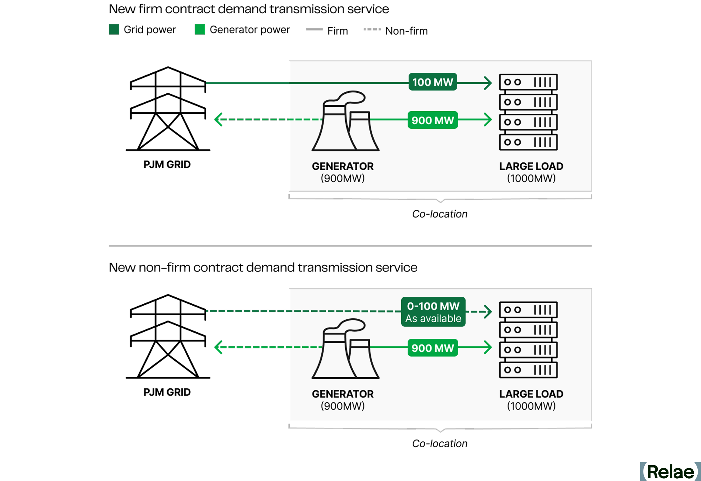
The interconnection mechanic (how the load connects) and the tariff product (what service the load receives) are two distinct decisions. For example, in the case of an interim NITS, a data center and co-located load could connect through a Provisional Interconnection Service (PIS). Other co-located loads may connect by submitting a request for acceleration at Decision Points I and II to secure firm contract demand service. The connection mechanism and tariff will vary based on each co-located load’s unique characteristics and project configuration. 

For clients evaluating specific sites, the right path depends on how much of the host generator's interconnection capacity is available, how sensitive the load is to interruption, and how fast the site needs to energize. Grid modeling allows project teams to quantitatively assess their risk exposure before committing to a tariff product. 

Which Two PJM Proposals Did FERC Reject?

Two elements of PJM's original filing did not make it through the April 16 order.

1. Point of Change in Ownership substitution: PJM proposed swapping in "Point of Change in Ownership" for FERC’s mandated term "Point of Interconnection" in the definition of Co-Located Load. FERC rejected the swap as an unexplained deviation from the Co-Location Order's definition and because it could let transmission owners delay or effectively veto the Point of Change in Ownership location, creating uncertainty for co-located projects.
2. BTM application-rule changes: PJM tried to fold changes to its BTM application rules into this same compliance package. FERC rejected that on the ground the changes did not fall within the scope of the initial order. BTM remains a separate regulatory track; the April 16 order does not settle it.

Project configurations built on either rejected proposal need restructuring before PJM's May 18 refile.

The order also directs PJM to add the PIS definition to the Open Access Transmission Tariff (OATT), Part I, section 1 (paragraph 26), and flags items in paragraph 29, including assessment of the reliability of co-located loads paired with electric storage, as out of scope. 

These determinations should not be seen as FERC rejecting these tariff changes, but rather deeming them outside the scope of the order. They are open questions that belong in a separate docket. The direction to include PIS while declining to address issues not included in the compliance proceeding demonstrates FERC’s focus on speed-to-power, clarifying the rules for new co-located generators to connect to the grid more quickly.  

What Is the Two-Strike Reliability Rule, and Why Does it Matter?

The rules for violating a co-location interconnection service agreement are still being developed, but FERC has urged PJM to issue robust protections to maintain reliability and cost allocation equity. 

For both firm and non-firm contract demand transmission service, PJM will apply a penalty rate to transmission service customers who withdraw more energy from the grid than was contracted. The precise design of these rates for unreserved use is scheduled for a paper hearing this spring; however, developers should cautiously size and appropriately model load and generation sizes, as the penalties for jeopardizing PJM’s reliability are not limited to rates. 

While penalty rate design for unreserved use is underway, PJM proposed a strict Two-Strike reliability rule for co-located projects. If a co-located customer failed to adequately implement automated loadshedding or generator tripping mechanisms during unusual grid conditions, PJM has previewed severe consequences:  

• First strike: a 120-day operational pause for review.
• Second strike: termination of the transmission service contract and return to the NITS interconnection waitlist.

The entire purpose of pursuing a co-located large load configuration is to ensure speed-to-power while maintaining reliability. In a June 2026 order, FERC conceded that there are legitimate reliability concerns with co-located generation misoperation; however, PJM’s proposal to disqualify customers with multiple misoperations is unnecessarily strict. FERC ultimately agreed PJM has the authority to charge penalties to and temporarily suspend services for customers that fail to shed load or curtail, but cannot disqualify customers for misoperation. Data centers will need to rigorously model and design their co-located load and generator facilities with the understanding that multiple reliability violations could strand billion-dollar assets for multiple years. 

Which BYOG Deals Need Restructuring Before the May 18 Refile?

Any deal built around the Point of Change in Ownership substitution or the BTM application-rule changes that FERC rejected needs restructuring. 

In addition, co-located projects that relied on one of the four approved mechanics, but used PJM tariff language from the original December filing, may also need re-papering against the language PJM submits in its forthcoming May 18 compliance filing. Until PJM files that package and FERC accepts it, the operative document is the April 16 order itself.

Counterparties should confirm that operational controls, curtailment rights, and dispute mechanisms in the contract align with the proposed Two-Strike regime and the approved mechanics the project uses.

What Does Grid Modeling Reveal for a Co-Located Project?

Non-firm service is the lowest-cost tariff product for the portion of load the co-located generator does not serve, but availability depends on real-time grid conditions. Grid modeling is how developers size that exposure before signing.

Take the same 1,000 MW data center paired with a 900 MW on-site generator, contracting 100 MW of non-firm service for the residual load. Grid modeling might show non-firm power dropping out in roughly 15% of hours during the summer peak.

If the on-site generator also carries a 5% forced outage rate, the developer faces a meaningful probability of a compound event: grid supply drops out at the same moment the on-site unit trips offline.

In that window, the data center has three options, none of them free: 

1. Curtail load. 
2. Shift the load to another site. 
3. Draw more from the grid than the contract allows, which triggers a Two-Strike violation.

Grid modeling converts that risk into decisions the developer can price. A developer can test whether adding 50 MW of battery storage, contracting 150 MW of firm service instead of 100 MW of non-firm, or adding a smaller backup generator delivers the best risk-adjusted return.

Key Takeaways

• Accurate load forecasting is needed to distinguish and prioritize real demand, align capital deployment, and reduce delays in bringing new power capacity online. Traditional load forecasting was built for predictable, gradual demand growth, not for the scale, uncertainty, and dynamic behavior of data centers. 
• The system-level fix to data-center load forecasting requires probabilistic, more frequent, category-specific methods paired with mandatory data standards and policy alignment. Together, these give planners visibility into the range of possible futures and the likelihood of each. 
• Without that fix, today's forecasts conflate real demand with speculative submissions, reducing accuracy. Inaccurate forecasting in either direction is expensive: underbuild adds friction to economic development; overbuild risks raising retail rates. Both can erode public trust in planning.
• Behind-the-meter generation (BTM) and load flexibility can help achieve speed-to-power in the near term. Just 1% data-center flexibility could unlock 100 GW—more than the entire US nuclear fleet.

Load Growth Is Increasing, Uncertain, and Concentrated

For two decades, US electricity demand was flat. Utilities, transmission planners, and corporate buyers built their planning models around that reality. Then AI workloads changed it.

AI load growth is large, uncertain, and concentrated in major power markets. While load forecasting projections vary across studies, the trajectory is clear: electricity demand is scaling faster than the bulk power grid was designed to handle. Accurate load forecasting is needed to distinguish and prioritize real demand, align capital deployment, and reduce delays in bringing new power capacity online.

On April 30, 2026, Relae (formerly Carbon Direct) hosted a Trellis Group panel on load forecasting in the AI era. Panelists included Derya Eryilmaz, PhD, Vice President of Power Commercialization at Relae; John Miller, Director of Transmission Policy at the Corporate Energy Buyers Association (CEBA); Daniel Padilla, Strategy and Business Development Lead at Emerald AI; and Sam Hodas, Head of US Government Affairs at National Grid. Jake Mitchell, Director of Climate Tech Innovation at Trellis Group, moderated.

The conversation explored where load forecasts fail, what they cost, how to fix them, and near-term solutions to overcome grid constraints. Here is what the panel found.

What Is Load Forecasting?

Load forecasting is the practice of predicting how much electricity will be consumed across a region, at what times, and under what conditions. It informs the major capital and procurement decisions on the grid: where to build transmission, how much generation to procure, what capacity to bid into wholesale markets, and how corporate buyers secure clean, firm power.

Long-term forecasts inform multi-year decisions about transmission and generation. Short-term operational forecasts inform real-time grid operations and trading. The two often sit in separate workflows, but short-term operational forecasts should feed into long-term system planning to improve accuracy as demand patterns shift.

The Bulk Power Grid Is Under Strain

Large power users face constraints on clean, firm power, transmission capacity, multi-year interconnection queues, and aging infrastructure. The strain is most acute in PJM Interconnection (PJM) and the Electric Reliability Council of Texas (ERCOT), the two US markets expected to see the most significant load growth. Each constraint raises the cost of getting load forecasts wrong.

Hodas from National Grid describes the operational reality on the utility side: aging infrastructure inherited from a different demand era. “We’ve got transmission lines that are 70 to 100 years old in New York and Massachusetts, some of the oldest in the country, still in operation.” Replacing or upgrading that infrastructure requires investment, and ratepayers are already pressed. 

Why Today’s Load Forecasts Fail

Traditional load forecasting was built for predictable, gradual demand growth, not for the scale, uncertainty, and dynamic behavior of data centers. 

Most utilities and Independent System Operators (ISOs) produce load forecasts on annual or biannual cycles. They aggregate submissions from individual customers, run that data through a deterministic single-peak load estimate against a single capacity scenario, and pass the consolidated forecast up to regional planners. Regional Transmission Organizations (RTOs) roll those bottom-up utility forecasts into a regional view. 

This worked when demand was flat and predictable. It no longer works with nonlinear growth driven by data centers. Eryilmaz from Relae identifies key structural limitations. 

Four Structural Limitations to Traditional Forecasting Methods

• Over-stating and double-counting. Data centers bid into multiple regions while shopping for power, inflating regional forecasts and blurring the line between real and hypothetical demand—the speculative-load problem.
• Deterministic models (vs probabilistic models). Most planning runs a single peak load estimate against a single capacity scenario, missing the geographic concentration and uncertainty inherent in integrating large loads into the system.
• Aggregated submissions. Utilities report large loads as a single block of gigawatts, with no resolution into workload type, ramp schedule, or operational shape. Planners reverse-engineer peak-demand assumptions rather than measure them.
• Infrequent cadence. Annual or biannual forecasts cannot catch an 80% queue reduction or a multi-gigawatt addition between cycles.

The Speculative-Load Problem

The core challenge in load forecasting is distinguishing real versus hypothetical load. While data center electricity demand is projected to grow by 13-27% annually through 2028, the majority of the projects in the data center queue may not materialize, inflating regional load forecasts.

American Electric Power's Ohio utility (AEP Ohio) introduced a tariff requiring data centers to put up firm financial commitments before getting in line for grid connection. Its interconnection queue dropped from 30 gigawatts to 5.6 gigawatts. More than 80% of the submitted load was speculative: projects that disappeared once commitment became required.

ERCOT shows the same overstatement problem on a larger scale. Roughly 225 gigawatts of data center demand sits in the ERCOT queue against a historic system peak of 85 gigawatts. Texas Senate Bill 6 introduced similar financial obligations for new loads, but those rules apply only to interconnections after 2025, and the cleanup of speculative demand has not yet materialized.

The speculative-load problem shows up in interconnection times. An average new project in PJM can wait 4 to 5 years to become operational. Some of that delay is a real backlog. The rest comes from the inability to distinguish real submissions from speculative ones.

As Eryilmaz puts it, “Load forecasting is actually the center of all of these problems. It is a tool to help planners make the right investment decisions.”

The Cost of Inaccurate Forecasting

As Miller from CEBA notes, “A single misforecasted project can swing a transmission plan by hundreds of megawatts.” Significant inaccuracies can erode public trust in the planning process in two main ways. Underbuilding adds friction to economic development and can limit corporate access to clean power markets. Conversely, overbuilding risks raising retail rates if capacity remains underutilized. 

The goal is to achieve right-sized infrastructure investment. When planning aligns with actual large load growth, it can be net beneficial to retail rates. By spreading fixed costs across more usage, significant new demand can put downward pressure on the rates via the “denominator effect.” 

On the other hand, forecasting variability can distort capacity procurement and interconnection queue prioritization. When load forecasts spike upward, grid operators like PJM have to scramble to buy additional electricity capacity on short notice. These emergency procurements lock in major dollar commitments on the basis of unstable forecast numbers. 

PJM, Midcontinent Independent System Operator (MISO), and Southwest Power Pool (SPP) have also reshaped their interconnection queues to make room for new large loads, but those queue priorities depend on the same forecasts that are unreliable in the first place. 

“There is no substitute for good backbone regional transmission planning,” Miller says. “Full stop. That is the enabler of all of the load growth that we’re talking about.”

BTM Generation and Load Flexibility: A Near-Term Bridge

Hyperscalers’ need for power is way faster than that of utilities and RTOs. Generation alone cannot scale fast enough to meet this new demand, and hyperscalers need speed-to-power.

As Eryilmaz frames it, behind-the-meter generation and load flexibility are interim solutions to the timing mismatch between data center urgency and the grid's slower build cycles. BTM generation and flexibility work differently:

• BTM is power generated on the data center's side of the utility meter, bypassing grid interconnection entirely. The structure gives operators large, reliable blocks of power without waiting years for grid approval.
• Load flexibility is the demand-side approach. A data center modifies its grid draw in response to grid signals. In practice, that can mean curtailing compute workloads during stress events, pre-cooling facilities ahead of a heat wave, drawing from on-site batteries or generators, or shifting workloads to data centers in less-constrained regions.

The Value of Load Flexibility

Relae’s power system modeling quantifies the dollar value of load flexibility in ERCOT. Load flexibility can eliminate forced load shedding risk, even at 40 gigawatts of data center buildout, preventing $5.5 billion in annual consumer welfare losses by curtailing an average of 5% of demand for under 1% of operating hours.

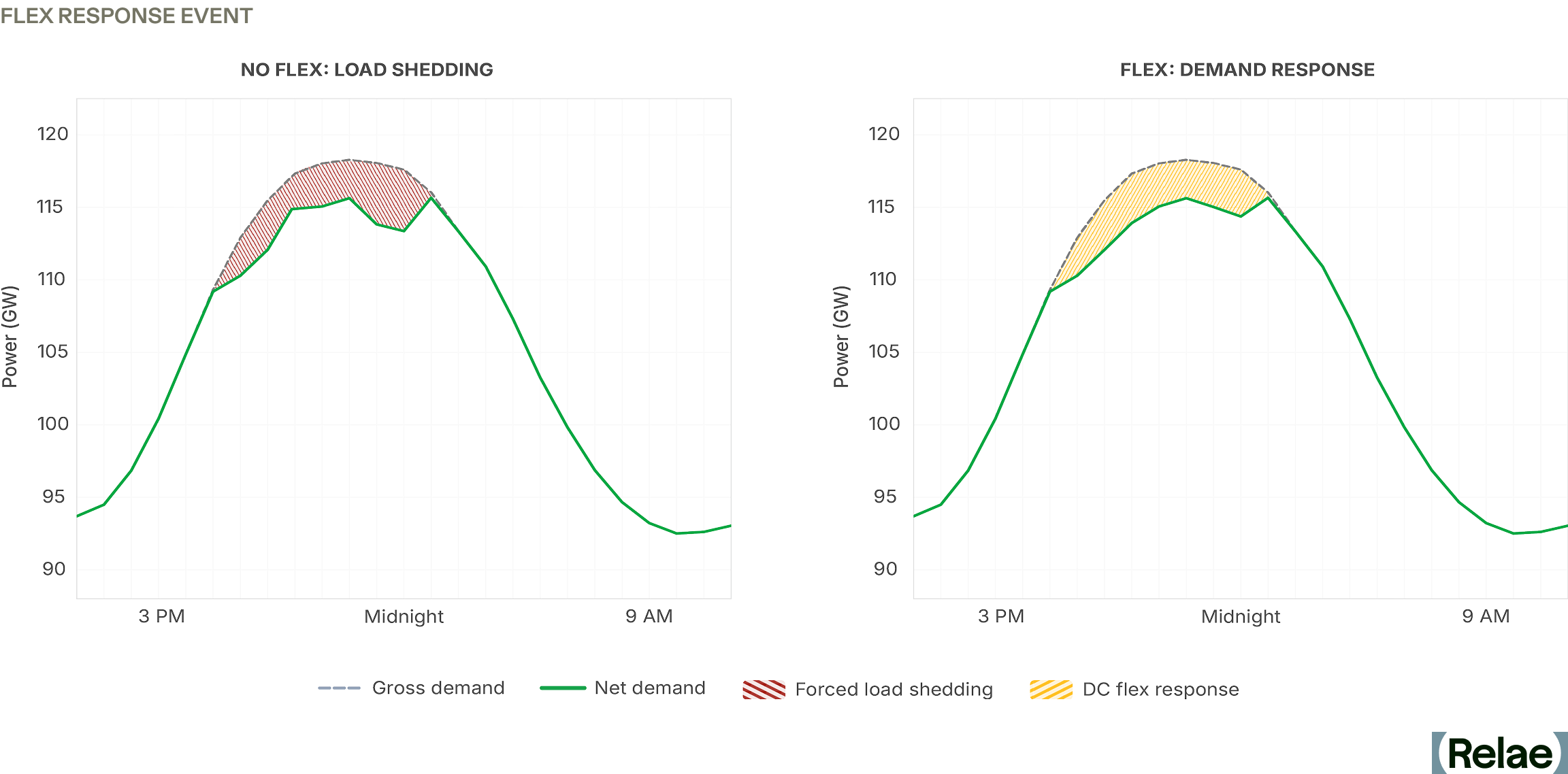
Padilla from Emerald AI reinforces the scale and value of load flexibility: “With just 1% flexibility, we can unlock 100 gigawatts of data centers across the US. That’s more than the entire US nuclear fleet.”

Silicon Valley Power, a municipal utility, is the first US utility to tie flexibility to interconnection speed: flexible data centers get connected faster. NVIDIA, EPRI, Digital Realty, and PJM are partnering on the Aurora AI Factory, the first purpose-built reference design for flexible AI data centers. 

But standardized policy for load flexibility is lagging. Padilla highlights this challenge: “Today, if a data center wants to be flexible, they have nowhere to point. We need standardized tariffs, interconnection rules, and product definitions for large loads that reward them with upsizing interconnection in response to flexibility.” 

Flexibility Takes Many Forms, but it Isn't Universal

Flexibility means accepting brief, predictable downtime, and some workloads can't tolerate it. Hospital systems and mission-critical enterprise applications need 99.999% uptime, the "five nines" standard. As Padilla puts it: "99.9% uptime, with brief and predictable curtailments, is plenty" for most AI workloads. That distinction determines which data centers can participate in flexibility programs.

Miller points out that compute-level flexibility is not always feasible. BTM batteries and virtual power plants (VPPs) are among the alternatives that can offset what data centers withdraw when the grid is stressed, even at facilities whose compute workloads cannot pause directly.

Better Load Forecasting: The Longer-Term Fix

While BTM generation and load flexibility can help address near-term speed-to-power, the longer-term fix is improving load forecasting methods and the standardization of data provided by the data centers themselves.

Eryilmaz outlines three technical shifts for better load forecasting:

• Embed short-term operational forecasting into long-term planning. Short-term spikes, weather risk, and reserve considerations carry direct implications for multi-year capital decisions. The line between operations and planning breaks down when growth is nonlinear.
• Replace deterministic models with probabilistic methods. Risk metrics like loss of load hours (expected hours per year that demand exceeds supply) and expected unserved energy (total expected energy shortfall) measure both how much capacity the system has and the conditions under which it might fall short. The North American Electric Reliability Corporation (NERC) has suggested both metrics as part of its reliability framework.
• Forecast load by category. Treating all data center load as a single block hides the differences in load profiles, operational schedules, and ramp-up timing that drive system planning.

Policy Alignment

Technical forecasting improvements only scale with policy alignment, and Miller proposes a two-part fix:

On the top-down side, RTOs need authority to take an independent view of utility-submitted forecasts. They should require milestones, such as firm financial commitments and secured financing, before counting a submitted load against the regional forecast. 

On the bottom-up side, state regulators set the rules that govern how individual utilities prepare their forecasts. Large load tariffs play a big role in how utility-level forecasts come together. Federal and state authorities need to row in the same direction. Hodas frames the same alignment from the utility side: “Grid investment unlocks economic growth, but for us to make those investments, we need regulatory certainty.”

Standardizing Large-Load Data

The Federal Energy Regulatory Commission (FERC) has since moved: in June 2026 it issued show cause orders directing six RTOs and ISOs—CAISO, ISO-NE, MISO, NYISO, PJM, and SPP—to revise or justify their large-load interconnection rules, and in July 2026 it directed NERC to develop computational-load reliability standards and registration criteria by the end of the year. Both are useful first steps. But as Eryilmaz argues, voluntary disclosure has not closed the gap.

The industry cannot meaningfully compare ISO forecasts when each utility submits load data in different shapes (e.g., using different methods and data standards) on different schedules. Mandatory submission requirements and published methodologies, applied consistently across utilities, ISOs, and state regulators, are the only path to forecasts whose components are actually comparable.

Getting Load Forecasting Right Starts Now

The system-level fix to improving forecasting is through probabilistic, category-specific methods paired with data standardization and policy support. Together, these account for the scale, uncertainty, and dynamic behavior of data center loads, and give planners visibility into the range of possible futures and the likelihood of each.  

All forecasts will be wrong to some degree, but as Miller puts it, “It's ultimately not about having a perfect prediction. It's about baking in methods to account for uncertainty.” These system-level improvements won't eliminate errors entirely, but they will minimize them, leading to more confident investment decisions and a grid better prepared for what's ahead.

Frequently Asked Questions

What is load forecasting, and why is it harder now with AI data center loads?

Load forecasting predicts how much electricity a region will consume, when, and under what conditions—the basis for where to build transmission, how much generation to procure, and how corporate buyers secure clean, firm power. It was designed for two decades of flat, gradual demand growth. Data center load is none of those things: it is large, geographically concentrated, arrives in gigawatt blocks with no disclosed operating shape, and can be withdrawn as quickly as it appeared.

What is speculative load in an interconnection queue, and how do planners tell it apart from real demand?

Speculative load is capacity requested by projects that may never be built — often the same data center bidding into several regions at once while shopping for power, which counts the same gigawatts more than once. The tested filter is a financial commitment: when AEP Ohio required firm commitments before queue entry, the utility's reported data center pipeline fell from about 30 GW to roughly 5.7 GW. Milestone requirements, independent RTO review of utility submissions, and mandatory data standards are the tools planners have.

Is load flexibility proven and scalable today, or still emerging?

The modeling case for load flexibility is strong; the commercial case is still early. Duke's Nicholas Institute found the 22 largest US balancing authority areas could absorb roughly 76–126 GW of new load if it accepts modest curtailment, and Relae's ERCOT modeling shows demand response eliminating forced load shedding risk at 40 GW of data center buildout, avoiding $5.5 billion in annual consumer welfare losses. What is still missing is the market plumbing—standardized tariffs, interconnection rules, and product definitions—so a data center willing to be flexible has somewhere to sign up.

What should a company look for when evaluating a region's load forecast?

Ask whether the forecast is probabilistic or a single deterministic peak, how often it is refreshed, and whether large loads are broken out by category and operating shape rather than reported as one block of gigawatts. Then ask what milestone or financial commitment a project must clear before its megawatts count toward the forecast. A forecast that cannot answer those three questions cannot tell you how much of the queue ahead of you is real.

[cta]